Tutorial: One dimensional Helmotz equation using Periodic Boundary Conditions#

This tutorial presents how to solve with Physics-Informed Neural Networks (PINNs) a one dimensional Helmotz equation with periodic boundary conditions (PBC). We will train with standard PINN’s training by augmenting the input with periodic expasion as presented in An expert’s guide to training physics-informed neural networks.

First of all, some useful imports.

## routine needed to run the notebook on Google Colab
try:
  import google.colab
  IN_COLAB = True
except:
  IN_COLAB = False
if IN_COLAB:
  !pip install "pina-mathlab"

import torch
import matplotlib.pyplot as plt
plt.style.use('tableau-colorblind10')

from pina import Condition, Plotter
from pina.problem import SpatialProblem
from pina.operators import laplacian
from pina.model import FeedForward
from pina.model.layers import PeriodicBoundaryEmbedding  # The PBC module
from pina.solvers import PINN
from pina.trainer import Trainer
from pina.geometry import CartesianDomain
from pina.equation import Equation

The problem definition#

The one-dimensional Helmotz problem is mathematically written as:

\[\begin{split}\begin{cases} \frac{d^2}{dx^2}u(x) - \lambda u(x) -f(x) &= 0 \quad x\in(0,2)\\ u^{(m)}(x=0) - u^{(m)}(x=2) &= 0 \quad m\in[0, 1, \cdots]\\ \end{cases}\end{split}\]

In this case we are asking the solution to be \(C^{\infty}\) periodic with period \(2\), on the inifite domain \(x\in(-\infty, \infty)\). Notice that the classical PINN would need inifinite conditions to evaluate the PBC loss function, one for each derivative, which is of course infeasable… A possible solution, diverging from the original PINN formulation, is to use coordinates augmentation. In coordinates augmentation you seek for a coordinates transformation \(v\) such that \(x\rightarrow v(x)\) such that the periodicity condition \(u^{(m)}(x=0) - u^{(m)}(x=2) = 0 \quad, m\in[0, 1, \cdots]\) is satisfied.

For demonstration porpuses the problem specifics are \(\lambda=-10\pi^2\), and \(f(x)=-6\pi^2\sin(3\pi x)\cos(\pi x)\) which gives a solution that can be computed analytically \(u(x) = \sin(\pi x)\cos(3\pi x)\).

class Helmotz(SpatialProblem):
    output_variables = ['u']
    spatial_domain = CartesianDomain({'x': [0, 2]})

    def helmotz_equation(input_, output_):
        x = input_.extract('x')
        u_xx = laplacian(output_, input_, components=['u'], d=['x'])
        f = - 6.*torch.pi**2 * torch.sin(3*torch.pi*x)*torch.cos(torch.pi*x)
        lambda_ = - 10. * torch.pi ** 2
        return u_xx - lambda_ * output_ - f

    # here we write the problem conditions
    conditions = {
        'D': Condition(location=spatial_domain,
                       equation=Equation(helmotz_equation)),
    }

    def helmotz_sol(self, pts):
        return torch.sin(torch.pi * pts) * torch.cos(3. * torch.pi * pts)

    truth_solution = helmotz_sol

problem = Helmotz()

# let's discretise the domain
problem.discretise_domain(200, 'grid', locations=['D'])

As usual the Helmotz problem is written in PINA code as a class. The equations are written as conditions that should be satisfied in the corresponding domains. The truth_solution is the exact solution which will be compared with the predicted one. We used latin hypercube sampling for choosing the collocation points.

Solving the problem with a Periodic Network#

Any \(\mathcal{C}^{\infty}\) periodic function \(u : \mathbb{R} \rightarrow \mathbb{R}\) with period \(L\in\mathbb{N}\) can be constructed by composition of an arbitrary smooth function \(f : \mathbb{R}^n \rightarrow \mathbb{R}\) and a given smooth periodic function \(v : \mathbb{R} \rightarrow \mathbb{R}^n\) with period \(L\), that is \(u(x) = f(v(x))\). The formulation is generalizable for arbitrary dimension, see A method for representing periodic functions and enforcing exactly periodic boundary conditions with deep neural networks.

In our case, we rewrite \(v(x) = \left[1, \cos\left(\frac{2\pi}{L} x\right), \sin\left(\frac{2\pi}{L} x\right)\right]\), i.e the coordinates augmentation, and \(f(\cdot) = NN_{\theta}(\cdot)\) i.e. a neural network. The resulting neural network obtained by composing \(f\) with \(v\) gives the PINN approximate solution, that is \(u(x) \approx u_{\theta}(x)=NN_{\theta}(v(x))\).

In PINA this translates in using the PeriodicBoundaryEmbedding layer for \(v\), and any pina.model for \(NN_{\theta}\). Let’s see it in action!

# we encapsulate all modules in a torch.nn.Sequential container
model = torch.nn.Sequential(PeriodicBoundaryEmbedding(input_dimension=1,
                                         periods=2),
                            FeedForward(input_dimensions=3, # output of PeriodicBoundaryEmbedding = 3 * input_dimension
                                        output_dimensions=1,
                                        layers=[10, 10]))

As simple as that! Notice in higher dimension you can specify different periods for all dimensions using a dictionary, e.g. periods={'x':2, 'y':3, ...} would indicate a periodicity of \(2\) in \(x\), \(3\) in \(y\), and so on…

We will now sole the problem as usually with the PINN and Trainer class.

pinn = PINN(problem=problem, model=model)
trainer = Trainer(pinn, max_epochs=5000, accelerator='cpu', enable_model_summary=False) # we train on CPU and avoid model summary at beginning of training (optional)
trainer.train()

GPU available: True (mps), used: False
TPU available: False, using: 0 TPU cores
IPU available: False, using: 0 IPUs
HPU available: False, using: 0 HPUs

Trainer.fit stopped: max_epochs=5000 reached.

Epoch 4999: 100%|██████████| 1/1 [00:00<00:00, 155.47it/s, v_num=20, D_loss=0.0123, mean_loss=0.0123]

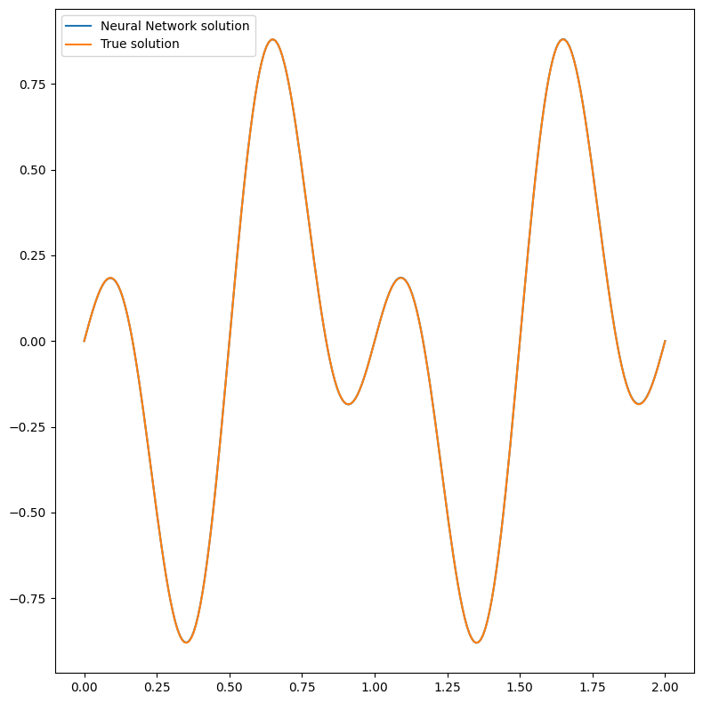
We are going to plot the solution now!

pl = Plotter()
pl.plot(pinn)

Great, they overlap perfectly! This seeams a good result, considering the simple neural network used to some this (complex) problem. We will now test the neural network on the domain \([-4, 4]\) without retraining. In principle the periodicity should be present since the \(v\) function ensures the periodicity in \((-\infty, \infty)\).

# plotting solution
with torch.no_grad():
    # Notice here we put [-4, 4]!!!
    new_domain = CartesianDomain({'x' : [0, 4]})
    x = new_domain.sample(1000, mode='grid')
    fig, axes = plt.subplots(1, 3, figsize=(15, 5))
    # Plot 1
    axes[0].plot(x, problem.truth_solution(x), label=r'$u(x)$', color='blue')
    axes[0].set_title(r'True solution $u(x)$')
    axes[0].legend(loc="upper right")
    # Plot 2
    axes[1].plot(x, pinn(x), label=r'$u_{\theta}(x)$', color='green')
    axes[1].set_title(r'PINN solution $u_{\theta}(x)$')
    axes[1].legend(loc="upper right")
    # Plot 3
    diff = torch.abs(problem.truth_solution(x) - pinn(x))
    axes[2].plot(x, diff, label=r'$|u(x) - u_{\theta}(x)|$', color='red')
    axes[2].set_title(r'Absolute difference $|u(x) - u_{\theta}(x)|$')
    axes[2].legend(loc="upper right")
    # Adjust layout
    plt.tight_layout()
    # Show the plots
    plt.show()

It is pretty clear that the network is periodic, with also the error following a periodic pattern. Obviusly a longer training, and a more expressive neural network could improve the results!

What’s next?#

Nice you have completed the one dimensional Helmotz tutorial of PINA! There are multiple directions you can go now:

Train the network for longer or with different layer sizes and assert the finaly accuracy
Apply the PeriodicBoundaryEmbedding layer for a time-dependent problem (see reference in the documentation)
Exploit extrafeature training ?
Many more…