Tutorial: Averaging Neural Operator for solving Kuramoto Sivashinsky equation#
In this tutorial we will build a Neural Operator using the
AveragingNeuralOperator model and the SupervisedSolver. At the
end of the tutorial you will be able to train a Neural Operator for
learning the operator of time dependent PDEs.
First of all, some useful imports. Note we use scipy for i/o
operations.
## routine needed to run the notebook on Google Colab
try:
  import google.colab
  IN_COLAB = True
except:
  IN_COLAB = False
if IN_COLAB:
  !pip install "pina-mathlab"
  !mkdir "data"
  !wget "https://github.com/mathLab/PINA/raw/refs/heads/master/tutorials/tutorial10/data/Data_KS.mat" -O "data/Data_KS.mat"
  !wget "https://github.com/mathLab/PINA/raw/refs/heads/master/tutorials/tutorial10/data/Data_KS2.mat" -O "data/Data_KS2.mat"


import torch
import matplotlib.pyplot as plt
plt.style.use('tableau-colorblind10')
from scipy import io
from pina import Condition, LabelTensor
from pina.problem import AbstractProblem
from pina.model import AveragingNeuralOperator
from pina.solvers import SupervisedSolver
from pina.trainer import Trainer
Data Generation#
We will focus on solving a specific PDE, the Kuramoto Sivashinsky (KS) equation. The KS PDE is a fourth-order nonlinear PDE with the following form:
In the above \(x\in \Omega=[0, 64]\) represents a spatial location, \(t\in\mathbb{T}=[0,50]\) the time and \(u(x, t)\) is the value of the function \(u:\Omega \times\mathbb{T}\in\mathbb{R}\). We indicate with \(\mathbb{U}\) a suitable space for \(u\), i.e. we have that the solution \(u\in\mathbb{U}\).
We impose Dirichlet boundary conditions on the derivative of \(u\) on the border of the domain \(\partial \Omega\)
Initial conditions are sampled from a distribution over truncated Fourier series with random coefficients \(\{A_k, \ell_k, \phi_k\}_k\) as
where \(A_k \in [-0.4, -0.3]\), \(\ell_k = 2\), \(\phi_k = 2\pi \quad \forall k=1,\dots,N\).
We have already generated some data for differenti initial conditions, and our objective will be to build a Neural Operator that, given \(u(x, t)\) will output \(u(x, t+\delta)\), where \(\delta\) is a fixed time step. We will come back on the Neural Operator architecture, for now we first need to import the data.
Note: The numerical integration is obtained by using pseudospectral method for spatial derivative discratization and implicit Runge Kutta 5 for temporal dynamics.
# load data
data=io.loadmat("dat/Data_KS.mat")

# converting to label tensor
initial_cond_train = LabelTensor(torch.tensor(data['initial_cond_train'], dtype=torch.float), ['t','x','u0'])
initial_cond_test = LabelTensor(torch.tensor(data['initial_cond_test'], dtype=torch.float), ['t','x','u0'])
sol_train = LabelTensor(torch.tensor(data['sol_train'], dtype=torch.float), ['u'])
sol_test = LabelTensor(torch.tensor(data['sol_test'], dtype=torch.float), ['u'])

print('Data Loaded')
print(f' shape initial condition: {initial_cond_train.shape}')
print(f' shape solution: {sol_train.shape}')
Data Loaded
 shape initial condition: torch.Size([100, 12800, 3])
 shape solution: torch.Size([100, 12800, 1])
The data are saved in the form B \times N \times D, where B is
the batch_size (basically how many initial conditions we sample), N
the number of points in the mesh (which is the product of the
discretization in x timese the one in t), and D the
dimension of the problem (in this case we have three variables
[u, t, x]).
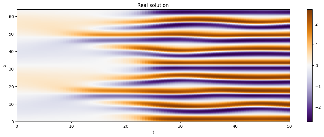
We are now going to plot some trajectories!
# helper function
def plot_trajectory(coords, real, no_sol=None):
    # find the x-t shapes
    dim_x = len(torch.unique(coords.extract('x')))
    dim_t = len(torch.unique(coords.extract('t')))
    # if we don't have the Neural Operator solution we simply plot the real one
    if no_sol is None:
        fig, axs = plt.subplots(1, 1, figsize=(15, 5), sharex=True, sharey=True)
        c = axs.imshow(real.reshape(dim_t, dim_x).T.detach(),extent=[0, 50, 0, 64], cmap='PuOr_r', aspect='auto')
        axs.set_title('Real solution')
        fig.colorbar(c, ax=axs)
        axs.set_xlabel('t')
        axs.set_ylabel('x')
    # otherwise we plot the real one, the Neural Operator one, and their difference
    else:
        fig, axs = plt.subplots(1, 3, figsize=(15, 5), sharex=True, sharey=True)
        axs[0].imshow(real.reshape(dim_t, dim_x).T.detach(),extent=[0, 50, 0, 64], cmap='PuOr_r', aspect='auto')
        axs[0].set_title('Real solution')
        axs[1].imshow(no_sol.reshape(dim_t, dim_x).T.detach(),extent=[0, 50, 0, 64], cmap='PuOr_r', aspect='auto')
        axs[1].set_title('NO solution')
        c = axs[2].imshow((real - no_sol).abs().reshape(dim_t, dim_x).T.detach(),extent=[0, 50, 0, 64], cmap='PuOr_r', aspect='auto')
        axs[2].set_title('Absolute difference')
        fig.colorbar(c, ax=axs.ravel().tolist())
        for ax in axs:
            ax.set_xlabel('t')
            ax.set_ylabel('x')
    plt.show()

# a sample trajectory (we use the sample 5, feel free to change)
sample_number = 20
plot_trajectory(coords=initial_cond_train[sample_number].extract(['x', 't']),
                real=sol_train[sample_number].extract('u'))

As we can see, as the time progresses the solution becomes chaotic,
which makes it really hard to learn! We will now focus on building a
Neural Operator using the SupervisedSolver class to tackle the
problem.
Averaging Neural Operator#
We will build a neural operator \(\texttt{NO}\) which takes the solution at time \(t=0\) for any \(x\in\Omega\), the time \((t)\) at which we want to compute the solution, and gives back the solution to the KS equation \(u(x, t)\), mathematically:
such that
There are many ways on approximating the following operator, e.g. by 2D FNO (for regular meshes), a DeepOnet, Continuous Convolutional Neural Operator, MIONet. In this tutorial we will use the Averaging Neural Operator presented in The Nonlocal Neural Operator: Universal Approximation which is a Kernel Neural Operator with integral kernel:
where:
\(v(x)\in\mathbb{R}^{\rm{emb}}\) is the update for a function \(v\) with \(\mathbb{R}^{\rm{emb}}\) the embedding (hidden) size
\(\sigma\) is a non-linear activation
\(W\in\mathbb{R}^{\rm{emb}\times\rm{emb}}\) is a tunable matrix.
\(b\in\mathbb{R}^{\rm{emb}}\) is a tunable bias.
If PINA many Kernel Neural Operators are already implemented, and the modular componets of the Kernel Neural Operator class permits to create new ones by composing base kernel layers.
Note:* We will use the already built class*
AveragingNeuralOperator, as constructive excercise try to use the
KernelNeuralOperator
class for building a kernel neural operator from scratch. You might
employ the different layers that we have in pina, e.g.
FeedForward,
and
AveragingNeuralOperator
layers.
class SIREN(torch.nn.Module):
    def forward(self, x):
        return torch.sin(x)

embedding_dimesion = 40     # hyperparameter embedding dimension
input_dimension = 3         # ['u', 'x', 't']
number_of_coordinates = 2   # ['x', 't']
lifting_net = torch.nn.Linear(input_dimension, embedding_dimesion)   # simple linear layers for lifting and projecting nets
projecting_net = torch.nn.Linear(embedding_dimesion + number_of_coordinates, 1)
model = AveragingNeuralOperator(lifting_net=lifting_net,
                                projecting_net=projecting_net,
                                coordinates_indices=['x', 't'],
                                field_indices=['u0'],
                                n_layers=4,
                                func=SIREN
                                )
Super easy! Notice that we use the SIREN activation function, more
on Implicit Neural Representations with Periodic Activation
Functions.
Solving the KS problem#
We will now focus on solving the KS equation using the
SupervisedSolver class and the AveragingNeuralOperator model. As
done in the FNO
tutorial
we now create the NeuralOperatorProblem class with
AbstractProblem.
# expected running time ~ 1 minute

class NeuralOperatorProblem(AbstractProblem):
    input_variables = initial_cond_train.labels
    output_variables = sol_train.labels
    conditions = {'data' : Condition(input_points=initial_cond_train,
                                     output_points=sol_train)}


# initialize problem
problem = NeuralOperatorProblem()
# initialize solver
solver = SupervisedSolver(problem=problem, model=model,optimizer_kwargs={"lr":0.001})
# train, only CPU and avoid model summary at beginning of training (optional)
trainer = Trainer(solver=solver, max_epochs=40, accelerator='cpu', enable_model_summary=False, log_every_n_steps=-1, batch_size=5) # we train on CPU and avoid model summary at beginning of training (optional)
trainer.train()
GPU available: True (mps), used: False
TPU available: False, using: 0 TPU cores
IPU available: False, using: 0 IPUs
HPU available: False, using: 0 HPUs
Epoch 39: 100%|██████████| 20/20 [00:01<00:00, 13.59it/s, v_num=3, mean_loss=0.118]
Trainer.fit stopped: max_epochs=40 reached.
Epoch 39: 100%|██████████| 20/20 [00:01<00:00, 13.56it/s, v_num=3, mean_loss=0.118]
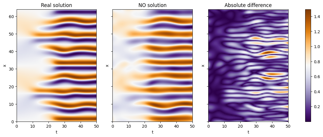
We can now see some plots for the solutions
sample_number = 2
no_sol = solver(initial_cond_test)
plot_trajectory(coords=initial_cond_test[sample_number].extract(['x', 't']),
                real=sol_test[sample_number].extract('u'),
                no_sol=no_sol[5])

As we can see we can obtain nice result considering the small trainint time and the difficulty of the problem! Let’s see how the training and testing error:
from pina.loss import PowerLoss

error_metric = PowerLoss(p=2)                                                   # we use the MSE loss

with torch.no_grad():
    no_sol_train = solver(initial_cond_train)
    err_train = error_metric(sol_train.extract('u'), no_sol_train).mean()       # we average the error over trajectories
    no_sol_test = solver(initial_cond_test)
    err_test = error_metric(sol_test.extract('u'),no_sol_test).mean()           # we average the error over trajectories
    print(f'Training error: {float(err_train):.3f}')
    print(f'Testing error: {float(err_test):.3f}')
Training error: 0.128
Testing error: 0.119
as we can see the error is pretty small, which agrees with what we can see from the previous plots.
What’s next?#
Now you know how to solve a time dependent neural operator problem in PINA! There are multiple directions you can go now:
Train the network for longer or with different layer sizes and assert the finaly accuracy
We left a more challenging dataset Data_KS2.mat where \(A_k \in [-0.5, 0.5]\), \(\ell_k \in [1, 2, 3]\), \(\phi_k \in [0, 2\pi]\) for loger training
Compare the performance between the different neural operators (you can even try to implement your favourite one!)
