Tutorial: Two dimensional Darcy flow using the Fourier Neural Operator#
In this tutorial we are going to solve the Darcy flow problem in two
dimensions, presented in Fourier Neural Operator for Parametric Partial
Differential Equation.
First of all we import the modules needed for the tutorial. Importing
scipy is needed for input output operations.
## routine needed to run the notebook on Google Colab
try:
  import google.colab
  IN_COLAB = True
except:
  IN_COLAB = False
if IN_COLAB:
  !pip install "pina-mathlab"
  !pip install scipy
  # get the data
  !wget https://github.com/mathLab/PINA/raw/refs/heads/master/tutorials/tutorial5/Data_Darcy.mat


# !pip install scipy  # install scipy
from scipy import io
import torch
from pina.model import FNO, FeedForward  # let's import some models
from pina import Condition, LabelTensor
from pina.solvers import SupervisedSolver
from pina.trainer import Trainer
from pina.problem import AbstractProblem
import matplotlib.pyplot as plt
plt.style.use('tableau-colorblind10')
Data Generation#
We will focus on solving the a specfic PDE, the Darcy Flow equation. The Darcy PDE is a second order, elliptic PDE with the following form:
Specifically, \(u\) is the flow pressure, \(k\) is the permeability field and \(f\) is the forcing function. The Darcy flow can parameterize a variety of systems including flow through porous media, elastic materials and heat conduction. Here you will define the domain as a 2D unit square Dirichlet boundary conditions. The dataset is taken from the authors original reference.
# download the dataset
data = io.loadmat("Data_Darcy.mat")

# extract data (we use only 100 data for train)
k_train = LabelTensor(torch.tensor(data['k_train'], dtype=torch.float).unsqueeze(-1), ['u0'])
u_train = LabelTensor(torch.tensor(data['u_train'], dtype=torch.float).unsqueeze(-1), ['u'])
k_test =  LabelTensor(torch.tensor(data['k_test'], dtype=torch.float).unsqueeze(-1), ['u0'])
u_test= LabelTensor(torch.tensor(data['u_test'], dtype=torch.float).unsqueeze(-1), ['u'])
x = torch.tensor(data['x'], dtype=torch.float)[0]
y = torch.tensor(data['y'], dtype=torch.float)[0]
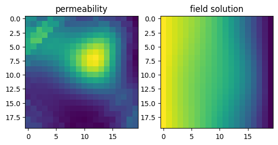
Let’s visualize some data
plt.subplot(1, 2, 1)
plt.title('permeability')
plt.imshow(k_train.squeeze(-1)[0])
plt.subplot(1, 2, 2)
plt.title('field solution')
plt.imshow(u_train.squeeze(-1)[0])
plt.show()

We now create the neural operator class. It is a very simple class,
inheriting from AbstractProblem.
class NeuralOperatorSolver(AbstractProblem):
    input_variables = k_train.labels
    output_variables = u_train.labels
    conditions = {'data' : Condition(input_points=k_train,
                                     output_points=u_train)}

# make problem
problem = NeuralOperatorSolver()
Solving the problem with a FeedForward Neural Network#
We will first solve the problem using a Feedforward neural network. We
will use the SupervisedSolver for solving the problem, since we are
training using supervised learning.
# make model
model = FeedForward(input_dimensions=1, output_dimensions=1)


# make solver
solver = SupervisedSolver(problem=problem, model=model)

# make the trainer and train
trainer = Trainer(solver=solver, max_epochs=10, accelerator='cpu', enable_model_summary=False, batch_size=10) # we train on CPU and avoid model summary at beginning of training (optional)
trainer.train()
GPU available: False, used: False
TPU available: False, using: 0 TPU cores
IPU available: False, using: 0 IPUs
HPU available: False, using: 0 HPUs
Epoch 9: : 100it [00:00, 357.28it/s, v_num=1, mean_loss=0.108]
Trainer.fit stopped: max_epochs=10 reached.
Epoch 9: : 100it [00:00, 354.81it/s, v_num=1, mean_loss=0.108]
The final loss is pretty high… We can calculate the error by importing
LpLoss.
from pina.loss import LpLoss

# make the metric
metric_err = LpLoss(relative=True)


err = float(metric_err(u_train.squeeze(-1), solver.neural_net(k_train).squeeze(-1)).mean())*100
print(f'Final error training {err:.2f}%')

err = float(metric_err(u_test.squeeze(-1), solver.neural_net(k_test).squeeze(-1)).mean())*100
print(f'Final error testing {err:.2f}%')
Final error training 56.04%
Final error testing 56.01%
Solving the problem with a Fuorier Neural Operator (FNO)#
We will now move to solve the problem using a FNO. Since we are learning operator this approach is better suited, as we shall see.
# make model
lifting_net = torch.nn.Linear(1, 24)
projecting_net = torch.nn.Linear(24, 1)
model = FNO(lifting_net=lifting_net,
            projecting_net=projecting_net,
            n_modes=8,
            dimensions=2,
            inner_size=24,
            padding=8)


# make solver
solver = SupervisedSolver(problem=problem, model=model)

# make the trainer and train
trainer = Trainer(solver=solver, max_epochs=10, accelerator='cpu', enable_model_summary=False, batch_size=10) # we train on CPU and avoid model summary at beginning of training (optional)
trainer.train()
GPU available: False, used: False
TPU available: False, using: 0 TPU cores
IPU available: False, using: 0 IPUs
HPU available: False, using: 0 HPUs
Epoch 0: : 0it [00:00, ?it/s]Epoch 9: : 100it [00:02, 47.76it/s, v_num=4, mean_loss=0.00106]
Trainer.fit stopped: max_epochs=10 reached.
Epoch 9: : 100it [00:02, 47.65it/s, v_num=4, mean_loss=0.00106]
We can clearly see that the final loss is lower. Let’s see in testing..
Notice that the number of parameters is way higher than a
FeedForward network. We suggest to use GPU or TPU for a speed up in
training, when many data samples are used.
err = float(metric_err(u_train.squeeze(-1), solver.neural_net(k_train).squeeze(-1)).mean())*100
print(f'Final error training {err:.2f}%')

err = float(metric_err(u_test.squeeze(-1), solver.neural_net(k_test).squeeze(-1)).mean())*100
print(f'Final error testing {err:.2f}%')
Final error training 4.83%
Final error testing 5.16%
As we can see the loss is way lower!
What’s next?#
We have made a very simple example on how to use the FNO for
learning neural operator. Currently in PINA we implement 1D/2D/3D
cases. We suggest to extend the tutorial using more complex problems and
train for longer, to see the full potential of neural operators.
