Tutorial: Physics Informed Neural Networks on PINA#
In this tutorial, we will demonstrate a typical use case of PINA on a toy problem, following the standard API procedure.
Specifically, the tutorial aims to introduce the following topics:
Explaining how to build PINA Problems,
Showing how to generate data for
PINNtraining
These are the two main steps needed before starting the modelling
optimization (choose model and solver, and train). We will show each
step in detail, and at the end, we will solve a simple Ordinary
Differential Equation (ODE) problem using the PINN solver.
Build a PINA problem#
Problem definition in the PINA framework is done by building a
python class, which inherits from one or more problem classes
(SpatialProblem, TimeDependentProblem, ParametricProblem, …)
depending on the nature of the problem. Below is an example:
Simple Ordinary Differential Equation#
Consider the following:
with the analytical solution \(u(x) = e^x\). In this case, our ODE
depends only on the spatial variable \(x\in(0,1)\) , meaning that
our Problem class is going to be inherited from the
SpatialProblem class:
from pina.problem import SpatialProblem
from pina.geometry import CartesianProblem

class SimpleODE(SpatialProblem):

    output_variables = ['u']
    spatial_domain = CartesianProblem({'x': [0, 1]})

    # other stuff ...
Notice that we define output_variables as a list of symbols,
indicating the output variables of our equation (in this case only
\(u\)), this is done because in PINA the torch.Tensors are
labelled, allowing the user maximal flexibility for the manipulation of
the tensor. The spatial_domain variable indicates where the sample
points are going to be sampled in the domain, in this case
\(x\in[0,1]\).
What if our equation is also time-dependent? In this case, our class
will inherit from both SpatialProblem and TimeDependentProblem:
## routine needed to run the notebook on Google Colab
try:
  import google.colab
  IN_COLAB = True
except:
  IN_COLAB = False
if IN_COLAB:
  !pip install "pina-mathlab"

from pina.problem import SpatialProblem, TimeDependentProblem
from pina.geometry import CartesianDomain

class TimeSpaceODE(SpatialProblem, TimeDependentProblem):

    output_variables = ['u']
    spatial_domain = CartesianDomain({'x': [0, 1]})
    temporal_domain = CartesianDomain({'t': [0, 1]})

    # other stuff ...
where we have included the temporal_domain variable, indicating the
time domain wanted for the solution.
In summary, using PINA, we can initialize a problem with a class
which inherits from different base classes: SpatialProblem,
TimeDependentProblem, ParametricProblem, and so on depending on
the type of problem we are considering. Here are some examples (more on
the official documentation):
SpatialProblem\(\rightarrow\) a differential equation with spatial variable(s)spatial_domainTimeDependentProblem\(\rightarrow\) a time-dependent differential equation with temporal variable(s)temporal_domainParametricProblem\(\rightarrow\) a parametrized differential equation with parametric variable(s)parameter_domainAbstractProblem\(\rightarrow\) any PINA problem inherits from here
Write the problem class#
Once the Problem class is initialized, we need to represent the
differential equation in PINA. In order to do this, we need to load
the PINA operators from pina.operators module. Again, we’ll
consider Equation (1) and represent it in PINA:
from pina.problem import SpatialProblem
from pina.operators import grad
from pina import Condition
from pina.geometry import CartesianDomain
from pina.equation import Equation, FixedValue

import torch


class SimpleODE(SpatialProblem):

    output_variables = ['u']
    spatial_domain = CartesianDomain({'x': [0, 1]})

    # defining the ode equation
    def ode_equation(input_, output_):

        # computing the derivative
        u_x = grad(output_, input_, components=['u'], d=['x'])

        # extracting the u input variable
        u = output_.extract(['u'])

        # calculate the residual and return it
        return u_x - u

    # conditions to hold
    conditions = {
        'x0': Condition(location=CartesianDomain({'x': 0.}), equation=FixedValue(1)),             # We fix initial condition to value 1
        'D': Condition(location=CartesianDomain({'x': [0, 1]}), equation=Equation(ode_equation)), # We wrap the python equation using Equation
    }

    # sampled points (see below)
    input_pts = None

    # defining the true solution
    def truth_solution(self, pts):
        return torch.exp(pts.extract(['x']))

problem = SimpleODE()
After we define the Problem class, we need to write different class
methods, where each method is a function returning a residual. These
functions are the ones minimized during PINN optimization, given the
initial conditions. For example, in the domain \([0,1]\), the ODE
equation (ode_equation) must be satisfied. We represent this by
returning the difference between subtracting the variable u from its
gradient (the residual), which we hope to minimize to 0. This is done
for all conditions. Notice that we do not pass directly a python
function, but an Equation object, which is initialized with the
python function. This is done so that all the computations and
internal checks are done inside PINA.
Once we have defined the function, we need to tell the neural network
where these methods are to be applied. To do so, we use the
Condition class. In the Condition class, we pass the location
points and the equation we want minimized on those points (other
possibilities are allowed, see the documentation for reference).
Finally, it’s possible to define a truth_solution function, which
can be useful if we want to plot the results and see how the real
solution compares to the expected (true) solution. Notice that the
truth_solution function is a method of the PINN class, but it is
not mandatory for problem definition.
Generate data#
Data for training can come in form of direct numerical simulation
results, or points in the domains. In case we perform unsupervised
learning, we just need the collocation points for training, i.e. points
where we want to evaluate the neural network. Sampling point in PINA
is very easy, here we show three examples using the
.discretise_domain method of the AbstractProblem class.
# sampling 20 points in [0, 1] through discretization in all locations
problem.discretise_domain(n=20, mode='grid', variables=['x'], locations='all')

# sampling 20 points in (0, 1) through latin hypercube sampling in D, and 1 point in x0
problem.discretise_domain(n=20, mode='latin', variables=['x'], locations=['D'])
problem.discretise_domain(n=1, mode='random', variables=['x'], locations=['x0'])

# sampling 20 points in (0, 1) randomly
problem.discretise_domain(n=20, mode='random', variables=['x'])
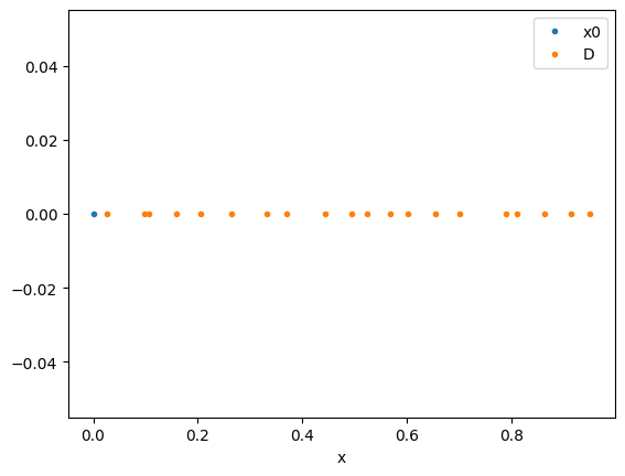
We are going to use latin hypercube points for sampling. We need to
sample in all the conditions domains. In our case we sample in D and
x0.
# sampling for training
problem.discretise_domain(1, 'random', locations=['x0'])
problem.discretise_domain(20, 'lh', locations=['D'])
The points are saved in a python dict, and can be accessed by
calling the attribute input_pts of the problem
print('Input points:', problem.input_pts)
print('Input points labels:', problem.input_pts['D'].labels)
Input points: {'x0': LabelTensor([[[0.]]]), 'D': LabelTensor([[[0.7644]],
             [[0.2028]],
             [[0.1789]],
             [[0.4294]],
             [[0.3239]],
             [[0.6531]],
             [[0.1406]],
             [[0.6062]],
             [[0.4969]],
             [[0.7429]],
             [[0.8681]],
             [[0.3800]],
             [[0.5357]],
             [[0.0152]],
             [[0.9679]],
             [[0.8101]],
             [[0.0662]],
             [[0.9095]],
             [[0.2503]],
             [[0.5580]]])}
Input points labels: ['x']
To visualize the sampled points we can use the .plot_samples method
of the Plotter class
from pina import Plotter

pl = Plotter()
pl.plot_samples(problem=problem)

Perform a small training#
Once we have defined the problem and generated the data we can start the
modelling. Here we will choose a FeedForward neural network
available in pina.model, and we will train using the PINN solver
from pina.solvers. We highlight that this training is fairly simple,
for more advanced stuff consider the tutorials in the Physics Informed
Neural Networks section of Tutorials. For training we use the
Trainer class from pina.trainer. Here we show a very short
training and some method for plotting the results. Notice that by
default all relevant metrics (e.g. MSE error during training) are going
to be tracked using a lightining logger, by default CSVLogger.
If you want to track the metric by yourself without a logger, use
pina.callbacks.MetricTracker.
from pina import Trainer
from pina.solvers import PINN
from pina.model import FeedForward
from pina.callbacks import MetricTracker


# build the model
model = FeedForward(
    layers=[10, 10],
    func=torch.nn.Tanh,
    output_dimensions=len(problem.output_variables),
    input_dimensions=len(problem.input_variables)
)

# create the PINN object
pinn = PINN(problem, model)

# create the trainer
trainer = Trainer(solver=pinn, max_epochs=1500, callbacks=[MetricTracker()], accelerator='cpu', enable_model_summary=False) # we train on CPU and avoid model summary at beginning of training (optional)

# train
trainer.train()
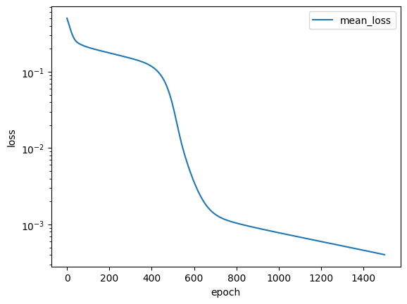
After the training we can inspect trainer logged metrics (by default
PINA logs mean square error residual loss). The logged metrics can
be accessed online using one of the Lightinig loggers. The final
loss can be accessed by trainer.logged_metrics
# inspecting final loss
trainer.logged_metrics
{'x0_loss': tensor(1.0674e-05),
 'D_loss': tensor(0.0008),
 'mean_loss': tensor(0.0004)}
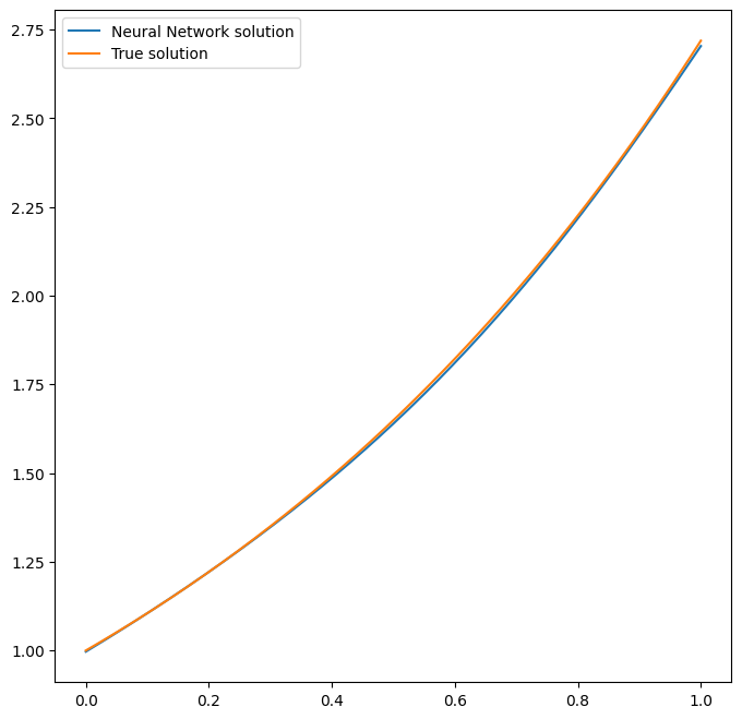
By using the Plotter class from PINA we can also do some
quatitative plots of the solution.
# plotting the solution
pl.plot(solver=pinn)

<Figure size 640x480 with 0 Axes>
The solution is overlapped with the actual one, and they are barely indistinguishable. We can also plot easily the loss:
pl.plot_loss(trainer=trainer, label = 'mean_loss', logy=True)

As we can see the loss has not reached a minimum, suggesting that we could train for longer
What’s next?#
Congratulations on completing the introductory tutorial of PINA! There are several directions you can go now:
Train the network for longer or with different layer sizes and assert the finaly accuracy
Train the network using other types of models (see
pina.model)GPU training and speed benchmarking
Many more…
