Tutorial: Two dimensional Wave problem with hard constraint#
In this tutorial we present how to solve the wave equation using hard
constraint PINNs. For doing so we will build a costum torch model
and pass it to the PINN solver.
First of all, some useful imports.
## routine needed to run the notebook on Google Colab
try:
  import google.colab
  IN_COLAB = True
except:
  IN_COLAB = False
if IN_COLAB:
  !pip install "pina-mathlab"

import torch

from pina.problem import SpatialProblem, TimeDependentProblem
from pina.operators import laplacian, grad
from pina.geometry import CartesianDomain
from pina.solvers import PINN
from pina.trainer import Trainer
from pina.equation import Equation
from pina.equation.equation_factory import FixedValue
from pina import Condition, Plotter
The problem definition#
The problem is written in the following form:
where \(D\) is a square domain \([0,1]^2\), and \(\Gamma_i\), with \(i=1,...,4\), are the boundaries of the square, and the velocity in the standard wave equation is fixed to one.
Now, the wave problem is written in PINA code as a class, inheriting
from SpatialProblem and TimeDependentProblem since we deal with
spatial, and time dependent variables. The equations are written as
conditions that should be satisfied in the corresponding domains.
truth_solution is the exact solution which will be compared with the
predicted one.
class Wave(TimeDependentProblem, SpatialProblem):
    output_variables = ['u']
    spatial_domain = CartesianDomain({'x': [0, 1], 'y': [0, 1]})
    temporal_domain = CartesianDomain({'t': [0, 1]})

    def wave_equation(input_, output_):
        u_t = grad(output_, input_, components=['u'], d=['t'])
        u_tt = grad(u_t, input_, components=['dudt'], d=['t'])
        nabla_u = laplacian(output_, input_, components=['u'], d=['x', 'y'])
        return nabla_u - u_tt

    def initial_condition(input_, output_):
        u_expected = (torch.sin(torch.pi*input_.extract(['x'])) *
                      torch.sin(torch.pi*input_.extract(['y'])))
        return output_.extract(['u']) - u_expected

    conditions = {
        'gamma1': Condition(location=CartesianDomain({'x': [0, 1], 'y':  1, 't': [0, 1]}), equation=FixedValue(0.)),
        'gamma2': Condition(location=CartesianDomain({'x': [0, 1], 'y': 0, 't': [0, 1]}), equation=FixedValue(0.)),
        'gamma3': Condition(location=CartesianDomain({'x':  1, 'y': [0, 1], 't': [0, 1]}), equation=FixedValue(0.)),
        'gamma4': Condition(location=CartesianDomain({'x': 0, 'y': [0, 1], 't': [0, 1]}), equation=FixedValue(0.)),
        't0': Condition(location=CartesianDomain({'x': [0, 1], 'y': [0, 1], 't': 0}), equation=Equation(initial_condition)),
        'D': Condition(location=CartesianDomain({'x': [0, 1], 'y': [0, 1], 't': [0, 1]}), equation=Equation(wave_equation)),
    }

    def wave_sol(self, pts):
        return (torch.sin(torch.pi*pts.extract(['x'])) *
                torch.sin(torch.pi*pts.extract(['y'])) *
                torch.cos(torch.sqrt(torch.tensor(2.))*torch.pi*pts.extract(['t'])))

    truth_solution = wave_sol

problem = Wave()
Hard Constraint Model#
After the problem, a torch model is needed to solve the PINN.
Usually, many models are already implemented in PINA, but the user
has the possibility to build his/her own model in torch. The hard
constraint we impose is on the boundary of the spatial domain.
Specifically, our solution is written as:
where \(NN\) is the neural net output. This neural network takes as
input the coordinates (in this case \(x\), \(y\) and \(t\))
and provides the unknown field \(u\). By construction, it is zero on
the boundaries. The residuals of the equations are evaluated at several
sampling points (which the user can manipulate using the method
discretise_domain) and the loss minimized by the neural network is
the sum of the residuals.
class HardMLP(torch.nn.Module):

    def __init__(self, input_dim, output_dim):
        super().__init__()

        self.layers = torch.nn.Sequential(torch.nn.Linear(input_dim, 40),
                                          torch.nn.ReLU(),
                                          torch.nn.Linear(40, 40),
                                          torch.nn.ReLU(),
                                          torch.nn.Linear(40, output_dim))

    # here in the foward we implement the hard constraints
    def forward(self, x):
        hard = x.extract(['x'])*(1-x.extract(['x']))*x.extract(['y'])*(1-x.extract(['y']))
        return hard*self.layers(x)
Train and Inference#
In this tutorial, the neural network is trained for 1000 epochs with a
learning rate of 0.001 (default in PINN). Training takes
approximately 3 minutes.
# generate the data
problem.discretise_domain(1000, 'random', locations=['D', 't0', 'gamma1', 'gamma2', 'gamma3', 'gamma4'])

# crete the solver
pinn = PINN(problem, HardMLP(len(problem.input_variables), len(problem.output_variables)))

# create trainer and train
trainer = Trainer(pinn, max_epochs=1000, accelerator='cpu', enable_model_summary=False) # we train on CPU and avoid model summary at beginning of training (optional)
trainer.train()
Trainer.fit stopped: max_epochs=1000 reached.
Epoch 999: : 1it [00:00, 68.69it/s, v_num=0, gamma1_loss=0.000, gamma2_loss=0.000, gamma3_loss=0.000, gamma4_loss=0.000, t0_loss=0.0419, D_loss=0.0307, mean_loss=0.0121]
Notice that the loss on the boundaries of the spatial domain is exactly
zero, as expected! After the training is completed one can now plot some
results using the Plotter class of PINA.
plotter = Plotter()

# plotting at fixed time t = 0.0
print('Plotting at t=0')
plotter.plot(pinn, fixed_variables={'t': 0.0})

# plotting at fixed time t = 0.5
print('Plotting at t=0.5')
plotter.plot(pinn, fixed_variables={'t': 0.5})

# plotting at fixed time t = 1.
print('Plotting at t=1')
plotter.plot(pinn, fixed_variables={'t': 1.0})
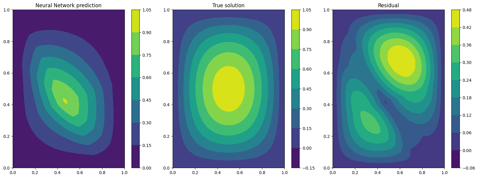
Plotting at t=0
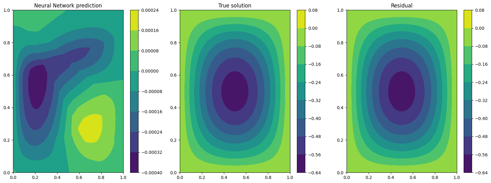
Plotting at t=0.5
Plotting at t=1
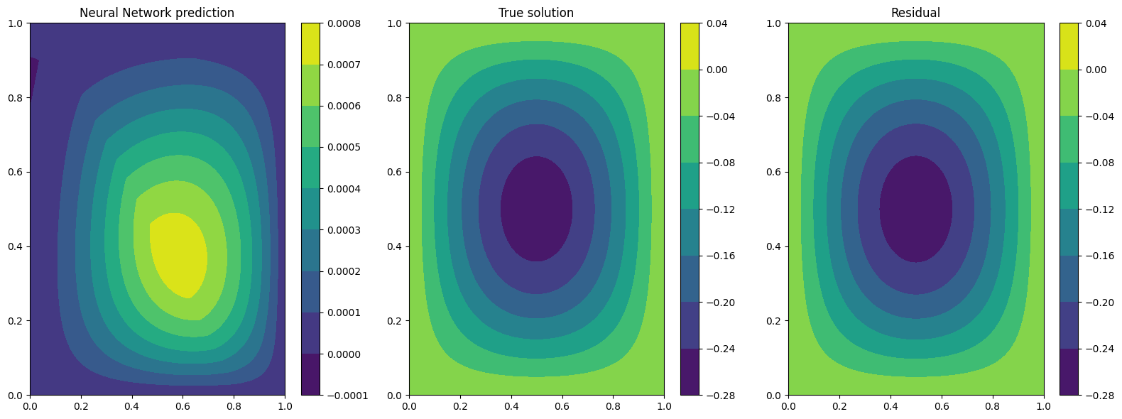
The results are not so great, and we can clearly see that as time progress the solution get worse…. Can we do better?
A valid option is to impose the initial condition as hard constraint as well. Specifically, our solution is written as:
Let us build the network first
class HardMLPtime(torch.nn.Module):

    def __init__(self, input_dim, output_dim):
        super().__init__()

        self.layers = torch.nn.Sequential(torch.nn.Linear(input_dim, 40),
                                          torch.nn.ReLU(),
                                          torch.nn.Linear(40, 40),
                                          torch.nn.ReLU(),
                                          torch.nn.Linear(40, output_dim))

    # here in the foward we implement the hard constraints
    def forward(self, x):
        hard_space = x.extract(['x'])*(1-x.extract(['x']))*x.extract(['y'])*(1-x.extract(['y']))
        hard_t = torch.sin(torch.pi*x.extract(['x'])) * torch.sin(torch.pi*x.extract(['y'])) * torch.cos(torch.sqrt(torch.tensor(2.))*torch.pi*x.extract(['t']))
        return hard_space * self.layers(x) * x.extract(['t']) + hard_t
Now let’s train with the same configuration as thre previous test
# generate the data
problem.discretise_domain(1000, 'random', locations=['D', 't0', 'gamma1', 'gamma2', 'gamma3', 'gamma4'])

# crete the solver
pinn = PINN(problem, HardMLPtime(len(problem.input_variables), len(problem.output_variables)))

# create trainer and train
trainer = Trainer(pinn, max_epochs=1000, accelerator='cpu', enable_model_summary=False) # we train on CPU and avoid model summary at beginning of training (optional)
trainer.train()
Trainer.fit stopped: max_epochs=1000 reached.
Epoch 999: : 1it [00:00, 45.78it/s, v_num=1, gamma1_loss=1.97e-15, gamma2_loss=0.000, gamma3_loss=2.14e-15, gamma4_loss=0.000, t0_loss=0.000, D_loss=1.25e-7, mean_loss=2.09e-8]
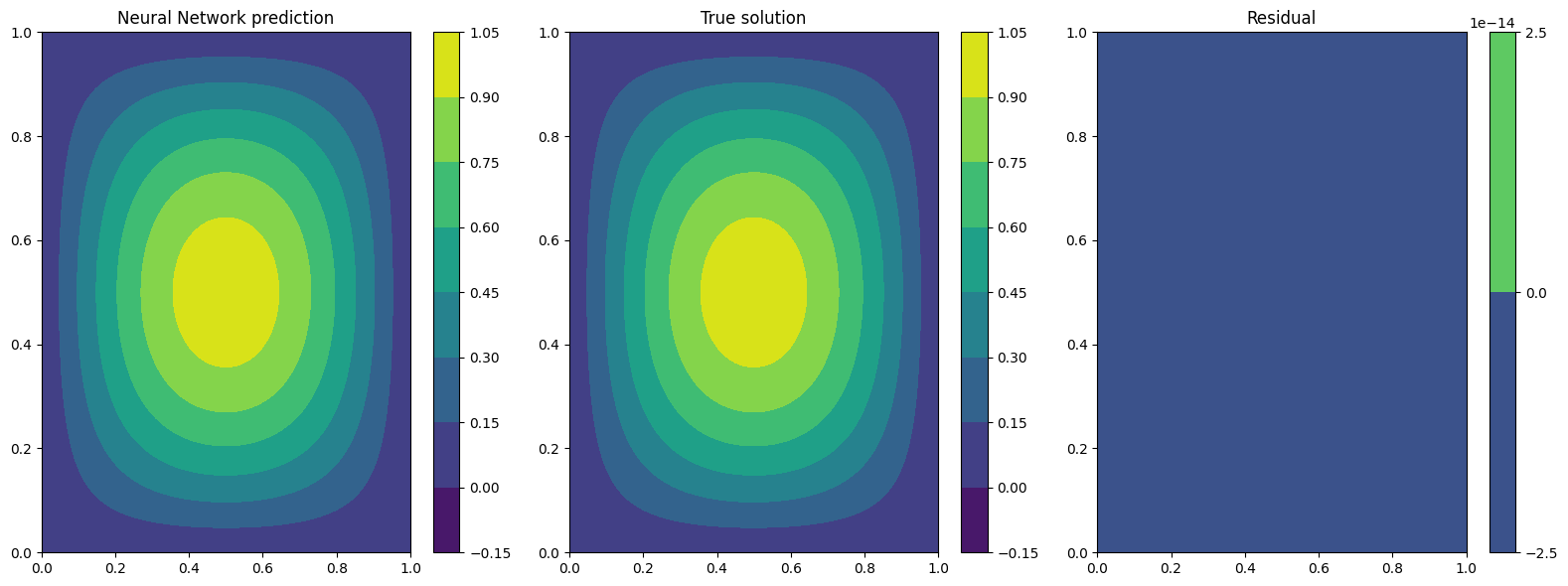
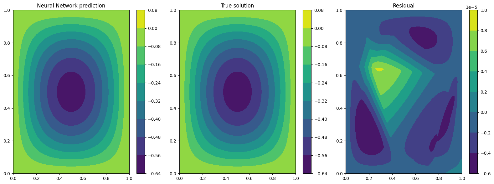
We can clearly see that the loss is way lower now. Let’s plot the results
plotter = Plotter()

# plotting at fixed time t = 0.0
print('Plotting at t=0')
plotter.plot(pinn, fixed_variables={'t': 0.0})

# plotting at fixed time t = 0.5
print('Plotting at t=0.5')
plotter.plot(pinn, fixed_variables={'t': 0.5})

# plotting at fixed time t = 1.
print('Plotting at t=1')
plotter.plot(pinn, fixed_variables={'t': 1.0})
Plotting at t=0
Plotting at t=0.5
Plotting at t=1
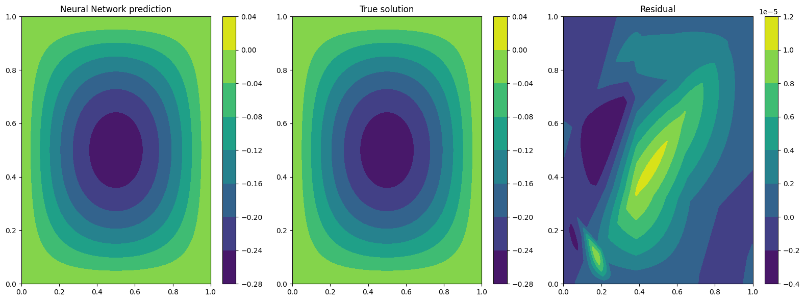
We can see now that the results are way better! This is due to the fact that previously the network was not learning correctly the initial conditon, leading to a poor solution when the time evolved. By imposing the initial condition the network is able to correctly solve the problem.
What’s next?#
Nice you have completed the two dimensional Wave tutorial of PINA! There are multiple directions you can go now:
Train the network for longer or with different layer sizes and assert the finaly accuracy
Propose new types of hard constraints in time, e.g.
\[u_{\rm{pinn}} = xy(1-x)(1-y)\cdot NN(x, y, t)(1-\exp(-t)) + \cos(\sqrt{2}\pi t)sin(\pi x)\sin(\pi y),\]Exploit extrafeature training for model 1 and 2
Many more…
