Tutorial: Resolution of an inverse problem#
Introduction to the inverse problem#
This tutorial shows how to solve an inverse Poisson problem with Physics-Informed Neural Networks. The problem definition is that of a Poisson problem with homogeneous boundary conditions and it reads:
where \(\Omega\) is a square domain \([-2, 2] \times [-2, 2]\), and \(\partial \Omega=\Gamma_1 \cup \Gamma_2 \cup \Gamma_3 \cup \Gamma_4\) is the union of the boundaries of the domain.
This kind of problem, namely the “inverse problem”, has two main goals:
find the solution \(u\) that satisfies the Poisson equation
find the unknown parameters (\(\mu_1\), \(\mu_2\)) that better fit some given data (third equation in the system above).
In order to achieve both the goals we will need to define an
InverseProblem in PINA. Let’s start with useful imports.
## routine needed to run the notebook on Google Colab
try:
  import google.colab
  IN_COLAB = True
except:
  IN_COLAB = False
if IN_COLAB:
  !pip install "pina-mathlab"
  # get the data
  !mkdir "data"
  !wget "https://github.com/mathLab/PINA/raw/refs/heads/master/tutorials/tutorial7/data/pinn_solution_0.5_0.5" -O "data/pinn_solution_0.5_0.5"
  !wget "https://github.com/mathLab/PINA/raw/refs/heads/master/tutorials/tutorial7/data/pts_0.5_0.5" -O "data/pts_0.5_0.5"


import matplotlib.pyplot as plt
plt.style.use('tableau-colorblind10')
import torch
from pytorch_lightning.callbacks import Callback
from pina.problem import SpatialProblem, InverseProblem
from pina.operators import laplacian
from pina.model import FeedForward
from pina.equation import Equation, FixedValue
from pina import Condition, Trainer
from pina.solvers import PINN
from pina.geometry import CartesianDomain
Then, we import the pre-saved data, for (\(\mu_1\),
\(\mu_2\))=(\(0.5\), \(0.5\)). These two values are the
optimal parameters that we want to find through the neural network
training. In particular, we import the input_points(the spatial
coordinates), and the output_points (the corresponding \(u\)
values evaluated at the input_points).
data_output = torch.load('data/pinn_solution_0.5_0.5').detach()
data_input = torch.load('data/pts_0.5_0.5')
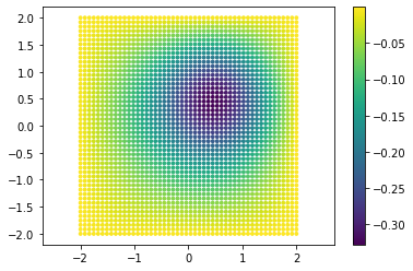
Moreover, let’s plot also the data points and the reference solution: this is the expected output of the neural network.
points = data_input.extract(['x', 'y']).detach().numpy()
truth = data_output.detach().numpy()

plt.scatter(points[:, 0], points[:, 1], c=truth, s=8)
plt.axis('equal')
plt.colorbar()
plt.show()

Inverse problem definition in PINA#
Then, we initialize the Poisson problem, that is inherited from the
SpatialProblem and from the InverseProblem classes. We here have
to define all the variables, and the domain where our unknown parameters
(\(\mu_1\), \(\mu_2\)) belong. Notice that the laplace equation
takes as inputs also the unknown variables, that will be treated as
parameters that the neural network optimizes during the training
process.
### Define ranges of variables
x_min = -2
x_max = 2
y_min = -2
y_max = 2

class Poisson(SpatialProblem, InverseProblem):
    '''
    Problem definition for the Poisson equation.
    '''
    output_variables = ['u']
    spatial_domain = CartesianDomain({'x': [x_min, x_max], 'y': [y_min, y_max]})
    # define the ranges for the parameters
    unknown_parameter_domain = CartesianDomain({'mu1': [-1, 1], 'mu2': [-1, 1]})

    def laplace_equation(input_, output_, params_):
        '''
        Laplace equation with a force term.
        '''
        force_term = torch.exp(
                - 2*(input_.extract(['x']) - params_['mu1'])**2
                - 2*(input_.extract(['y']) - params_['mu2'])**2)
        delta_u = laplacian(output_, input_, components=['u'], d=['x', 'y'])

        return delta_u - force_term

    # define the conditions for the loss (boundary conditions, equation, data)
    conditions = {
        'gamma1': Condition(location=CartesianDomain({'x': [x_min, x_max],
            'y':  y_max}),
            equation=FixedValue(0.0, components=['u'])),
        'gamma2': Condition(location=CartesianDomain({'x': [x_min, x_max], 'y': y_min
            }),
            equation=FixedValue(0.0, components=['u'])),
        'gamma3': Condition(location=CartesianDomain({'x':  x_max, 'y': [y_min, y_max]
            }),
            equation=FixedValue(0.0, components=['u'])),
        'gamma4': Condition(location=CartesianDomain({'x': x_min, 'y': [y_min, y_max]
            }),
            equation=FixedValue(0.0, components=['u'])),
        'D': Condition(location=CartesianDomain({'x': [x_min, x_max], 'y': [y_min, y_max]
            }),
        equation=Equation(laplace_equation)),
        'data': Condition(input_points=data_input.extract(['x', 'y']), output_points=data_output)
    }

problem = Poisson()
Then, we define the model of the neural network we want to use. Here we used a model which impose hard constrains on the boundary conditions, as also done in the Wave tutorial!
model = FeedForward(
    layers=[20, 20, 20],
    func=torch.nn.Softplus,
    output_dimensions=len(problem.output_variables),
    input_dimensions=len(problem.input_variables)
    )
After that, we discretize the spatial domain.
problem.discretise_domain(20, 'grid', locations=['D'], variables=['x', 'y'])
problem.discretise_domain(1000, 'random', locations=['gamma1', 'gamma2',
    'gamma3', 'gamma4'], variables=['x', 'y'])
Here, we define a simple callback for the trainer. We use this callback
to save the parameters predicted by the neural network during the
training. The parameters are saved every 100 epochs as torch tensors
in a specified directory (tmp_dir in our case). The goal is to read
the saved parameters after training and plot their trend across the
epochs.
# temporary directory for saving logs of training
tmp_dir = "tmp_poisson_inverse"

class SaveParameters(Callback):
    '''
    Callback to save the parameters of the model every 100 epochs.
    '''
    def on_train_epoch_end(self, trainer, __):
        if trainer.current_epoch % 100 == 99:
            torch.save(trainer.solver.problem.unknown_parameters, '{}/parameters_epoch{}'.format(tmp_dir, trainer.current_epoch))
Then, we define the PINN object and train the solver using the
Trainer.
### train the problem with PINN
max_epochs = 5000
pinn = PINN(problem, model, optimizer_kwargs={'lr':0.005})
# define the trainer for the solver
trainer = Trainer(solver=pinn, accelerator='cpu', max_epochs=max_epochs,
        default_root_dir=tmp_dir, callbacks=[SaveParameters()])
trainer.train()
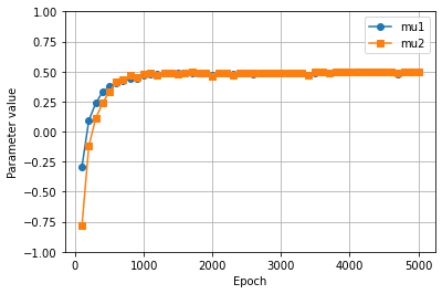
One can now see how the parameters vary during the training by reading the saved solution and plotting them. The plot shows that the parameters stabilize to their true value before reaching the epoch \(1000\)!
epochs_saved = range(99, max_epochs, 100)
parameters = torch.empty((int(max_epochs/100), 2))
for i, epoch in enumerate(epochs_saved):
    params_torch = torch.load('{}/parameters_epoch{}'.format(tmp_dir, epoch))
    for e, var in enumerate(pinn.problem.unknown_variables):
        parameters[i, e] = params_torch[var].data

# Plot parameters
plt.close()
plt.plot(epochs_saved, parameters[:, 0], label='mu1', marker='o')
plt.plot(epochs_saved, parameters[:, 1], label='mu2', marker='s')
plt.ylim(-1, 1)
plt.grid()
plt.legend()
plt.xlabel('Epoch')
plt.ylabel('Parameter value')
plt.show()

