Tutorial: Multiscale PDE learning with Fourier Feature Network#
This tutorial presents how to solve with Physics-Informed Neural Networks (PINNs) a PDE characterized by multiscale behaviour, as presented in On the eigenvector bias of Fourier feature networks: From regression to solving multi-scale PDEs with physics-informed neural networks.
First of all, some useful imports.
## routine needed to run the notebook on Google Colab
try:
  import google.colab
  IN_COLAB = True
except:
  IN_COLAB = False
if IN_COLAB:
  !pip install "pina-mathlab"

import torch

from pina import Condition, Plotter, Trainer, Plotter
from pina.problem import SpatialProblem
from pina.operators import laplacian
from pina.solvers import PINN, SAPINN
from pina.model.layers import FourierFeatureEmbedding
from pina.loss import LpLoss
from pina.geometry import CartesianDomain
from pina.equation import Equation, FixedValue
from pina.model import FeedForward
Multiscale Problem#
We begin by presenting the problem which also can be found in Section 2 of On the eigenvector bias of Fourier feature networks: From regression to solving multi-scale PDEs with physics-informed neural networks. The one-dimensional Poisson problem we aim to solve is mathematically written as:
We impose the solution as \(u(x) = \sin(2\pi x) + 0.1 \sin(50\pi x)\) and obtain the force term \(f(x) = (2\pi)^2 \sin(2\pi x) + 0.1 (50 \pi)^2 \sin(50\pi x)\). Though this example is simple and pedagogical, it is worth noting that the solution exhibits low frequency in the macro-scale and high frequency in the micro-scale, which resembles many practical scenarios.
In PINA this problem is written, as always, as a class see here for
a tutorial on the Problem
class.
Below you can find the Poisson problem which is mathmatically
described above.
class Poisson(SpatialProblem):
    output_variables = ['u']
    spatial_domain = CartesianDomain({'x': [0, 1]})

    def poisson_equation(input_, output_):
        x = input_.extract('x')
        u_xx = laplacian(output_, input_, components=['u'], d=['x'])
        f = ((2*torch.pi)**2)*torch.sin(2*torch.pi*x) + 0.1*((50*torch.pi)**2)*torch.sin(50*torch.pi*x)
        return u_xx + f

    # here we write the problem conditions
    conditions = {
        'gamma0' : Condition(location=CartesianDomain({'x': 0}),
                             equation=FixedValue(0)),
        'gamma1' : Condition(location=CartesianDomain({'x': 1}),
                             equation=FixedValue(0)),
        'D':       Condition(location=spatial_domain,
                             equation=Equation(poisson_equation)),
    }

    def truth_solution(self, x):
        return torch.sin(2*torch.pi*x) + 0.1*torch.sin(50*torch.pi*x)

problem = Poisson()

# let's discretise the domain
problem.discretise_domain(128, 'grid')
A standard PINN approach would be to fit this model using a Feed Forward (fully connected) Neural Network. For a conventional fully-connected neural network is easy to approximate a function \(u\), given sufficient data inside the computational domain. However solving high-frequency or multi-scale problems presents great challenges to PINNs especially when the number of data cannot capture the different scales.
Below we run a simulation using the PINN solver and the self
adaptive SAPINN solver, using a
FeedForward model. We used a MultiStepLR scheduler to decrease the learning rate
slowly during training (it takes around 2 minutes to run on CPU).
# training with PINN and visualize results
pinn = PINN(problem=problem,
            model=FeedForward(input_dimensions=1, output_dimensions=1, layers=[100, 100, 100]),
            scheduler=torch.optim.lr_scheduler.MultiStepLR,
            scheduler_kwargs={'milestones' : [1000, 2000, 3000, 4000], 'gamma':0.9})
trainer = Trainer(pinn, max_epochs=5000, accelerator='cpu', enable_model_summary=False)
trainer.train()

# training with PINN and visualize results
sapinn = SAPINN(problem=problem,
                model=FeedForward(input_dimensions=1, output_dimensions=1, layers=[100, 100, 100]),
                scheduler_model=torch.optim.lr_scheduler.MultiStepLR,
                scheduler_model_kwargs={'milestones' : [1000, 2000, 3000, 4000], 'gamma':0.9})
trainer_sapinn = Trainer(sapinn, max_epochs=5000, accelerator='cpu', enable_model_summary=False)
trainer_sapinn.train()

# plot results
pl = Plotter()
pl.plot(pinn, title='PINN Solution')
pl.plot(sapinn, title='Self Adaptive PINN Solution')
GPU available: True (mps), used: False
TPU available: False, using: 0 TPU cores
IPU available: False, using: 0 IPUs
HPU available: False, using: 0 HPUs
Epoch 4999: 100%|██████████| 1/1 [00:00<00:00, 97.66it/s, v_num=69, gamma0_loss=2.61e+3, gamma1_loss=2.61e+3, D_loss=409.0, mean_loss=1.88e+3]
GPU available: True (mps), used: False
TPU available: False, using: 0 TPU cores
IPU available: False, using: 0 IPUs
HPU available: False, using: 0 HPUs
Epoch 4999: 100%|██████████| 1/1 [00:00<00:00, 65.77it/s, v_num=70, gamma0_loss=151.0, gamma1_loss=148.0, D_loss=6.38e+5, mean_loss=2.13e+5]


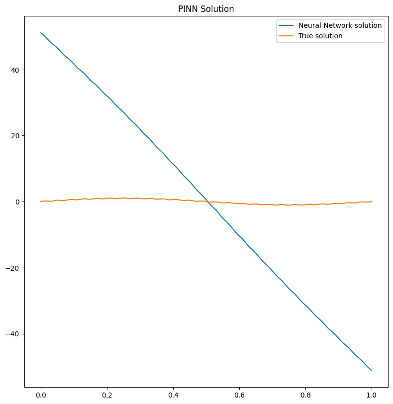
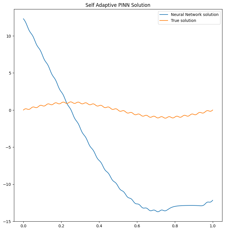
We can clearly see that the solution has not been learned by the two
different solvers. Indeed the big problem is not in the optimization
strategy (i.e. the solver), but in the model used to solve the problem.
A simple FeedForward network can hardly handle multiscales if not
enough collocation points are used!
We can also compute the \(l_2\) relative error for the PINN and
SAPINN solutions:
# l2 loss from PINA losses
l2_loss = LpLoss(p=2, relative=True)

# sample new test points
pts = pts = problem.spatial_domain.sample(100, 'grid')
print(f'Relative l2 error PINN      {l2_loss(pinn(pts), problem.truth_solution(pts)).item():.2%}')
print(f'Relative l2 error SAPINN    {l2_loss(sapinn(pts), problem.truth_solution(pts)).item():.2%}')
Relative l2 error PINN      95.76%
Relative l2 error SAPINN    124.26%
Which is indeed very high!
Fourier Feature Embedding in PINA#
Fourier Feature Embedding is a way to transform the input features, to help the network in learning multiscale variations in the output. It was first introduced in On the eigenvector bias of Fourier feature networks: From regression to solving multi-scale PDEs with physics-informed neural networks showing great results for multiscale problems. The basic idea is to map the input \(\mathbf{x}\) into an embedding \(\tilde{\mathbf{x}}\) where:
and \(\mathbf{B}_{ij} \sim \mathcal{N}(0, \sigma^2)\). This simple operation allow the network to learn on multiple scales!
In PINA we already have implemented the feature as a layer called
`FourierFeatureEmbedding <https://mathlab.github.io/PINA/_rst/layers/fourier_embedding.html>`__.
Below we will build the Multi-scale Fourier Feature Architecture. In
this architecture multiple Fourier feature embeddings (initialized with
different \(\sigma\)) are applied to input coordinates and then
passed through the same fully-connected neural network, before the
outputs are finally concatenated with a linear layer.
class MultiscaleFourierNet(torch.nn.Module):
    def __init__(self):
        super().__init__()
        self.embedding1 = FourierFeatureEmbedding(input_dimension=1,
                                                  output_dimension=100,
                                                  sigma=1)
        self.embedding2 = FourierFeatureEmbedding(input_dimension=1,
                                                  output_dimension=100,
                                                  sigma=10)
        self.layers = FeedForward(input_dimensions=100, output_dimensions=100, layers=[100])
        self.final_layer = torch.nn.Linear(2*100, 1)

    def forward(self, x):
        e1 = self.layers(self.embedding1(x))
        e2 = self.layers(self.embedding2(x))
        return self.final_layer(torch.cat([e1, e2], dim=-1))

MultiscaleFourierNet()
MultiscaleFourierNet(
  (embedding1): FourierFeatureEmbedding()
  (embedding2): FourierFeatureEmbedding()
  (layers): FeedForward(
    (model): Sequential(
      (0): Linear(in_features=100, out_features=100, bias=True)
      (1): Tanh()
      (2): Linear(in_features=100, out_features=100, bias=True)
    )
  )
  (final_layer): Linear(in_features=200, out_features=1, bias=True)
)
We will train the MultiscaleFourierNet with the PINN solver (and
feel free to try also with our PINN variants (SAPINN, GPINN,
CompetitivePINN, …).
multiscale_pinn = PINN(problem=problem,
                       model=MultiscaleFourierNet(),
                       scheduler=torch.optim.lr_scheduler.MultiStepLR,
                       scheduler_kwargs={'milestones' : [1000, 2000, 3000, 4000], 'gamma':0.9})
trainer = Trainer(multiscale_pinn, max_epochs=5000, accelerator='cpu', enable_model_summary=False) # we train on CPU and avoid model summary at beginning of training (optional)
trainer.train()
GPU available: True (mps), used: False
TPU available: False, using: 0 TPU cores
IPU available: False, using: 0 IPUs
HPU available: False, using: 0 HPUs
Epoch 4999: 100%|██████████| 1/1 [00:00<00:00, 72.21it/s, v_num=71, gamma0_loss=3.91e-5, gamma1_loss=3.91e-5, D_loss=0.000151, mean_loss=0.000113]
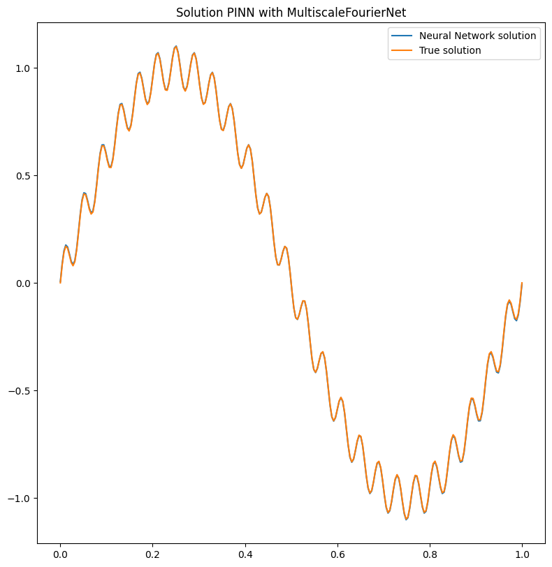
Let us now plot the solution and compute the relative \(l_2\) again!
# plot the solution
pl.plot(multiscale_pinn, title='Solution PINN with MultiscaleFourierNet')

# sample new test points
pts = pts = problem.spatial_domain.sample(100, 'grid')
print(f'Relative l2 error PINN with MultiscaleFourierNet      {l2_loss(multiscale_pinn(pts), problem.truth_solution(pts)).item():.2%}')

Relative l2 error PINN with MultiscaleFourierNet 2.72%
It is pretty clear that the network has learned the correct solution, with also a very law error. Obviously a longer training and a more expressive neural network could improve the results!
What’s next?#
Congratulations on completing the one dimensional Poisson tutorial of
PINA using FourierFeatureEmbedding! There are multiple
directions you can go now:
Train the network for longer or with different layer sizes and assert the finaly accuracy
Understand the role of
sigmainFourierFeatureEmbedding(see original paper for a nice reference)Code the Spatio-temporal multi-scale Fourier feature architecture for a more complex time dependent PDE (section 3 of the original reference)
Many more…
