Tutorial: Two dimensional Poisson problem using Extra Features Learning#
This tutorial presents how to solve with Physics-Informed Neural Networks (PINNs) a 2D Poisson problem with Dirichlet boundary conditions. We will train with standard PINN’s training, and with extrafeatures. For more insights on extrafeature learning please read An extended physics informed neural network for preliminary analysis of parametric optimal control problems.
First of all, some useful imports.
## routine needed to run the notebook on Google Colab
try:
  import google.colab
  IN_COLAB = True
except:
  IN_COLAB = False
if IN_COLAB:
  !pip install "pina-mathlab"

import torch
from torch.nn import Softplus

from pina.problem import SpatialProblem
from pina.operators import laplacian
from pina.model import FeedForward
from pina.solvers import PINN
from pina.trainer import Trainer
from pina.plotter import Plotter
from pina.geometry import CartesianDomain
from pina.equation import Equation, FixedValue
from pina import Condition, LabelTensor
from pina.callbacks import MetricTracker
The problem definition#
The two-dimensional Poisson problem is mathematically written as:
where \(D\) is a square domain \([0,1]^2\), and \(\Gamma_i\), with \(i=1,...,4\), are the boundaries of the square.
The Poisson problem is written in PINA code as a class. The equations are written as conditions that should be satisfied in the corresponding domains. The truth_solution is the exact solution which will be compared with the predicted one.
class Poisson(SpatialProblem):
    output_variables = ['u']
    spatial_domain = CartesianDomain({'x': [0, 1], 'y': [0, 1]})

    def laplace_equation(input_, output_):
        force_term = (torch.sin(input_.extract(['x'])*torch.pi) *
                      torch.sin(input_.extract(['y'])*torch.pi))
        laplacian_u = laplacian(output_, input_, components=['u'], d=['x', 'y'])
        return laplacian_u - force_term

    # here we write the problem conditions
    conditions = {
        'gamma1': Condition(location=CartesianDomain({'x': [0, 1], 'y':  1}), equation=FixedValue(0.)),
        'gamma2': Condition(location=CartesianDomain({'x': [0, 1], 'y': 0}), equation=FixedValue(0.)),
        'gamma3': Condition(location=CartesianDomain({'x':  1, 'y': [0, 1]}), equation=FixedValue(0.)),
        'gamma4': Condition(location=CartesianDomain({'x': 0, 'y': [0, 1]}), equation=FixedValue(0.)),
        'D': Condition(location=CartesianDomain({'x': [0, 1], 'y': [0, 1]}), equation=Equation(laplace_equation)),
    }

    def poisson_sol(self, pts):
        return -(
            torch.sin(pts.extract(['x'])*torch.pi)*
            torch.sin(pts.extract(['y'])*torch.pi)
        )/(2*torch.pi**2)

    truth_solution = poisson_sol

problem = Poisson()

# let's discretise the domain
problem.discretise_domain(25, 'grid', locations=['D'])
problem.discretise_domain(25, 'grid', locations=['gamma1', 'gamma2', 'gamma3', 'gamma4'])
Solving the problem with standard PINNs#
After the problem, the feed-forward neural network is defined, through
the class FeedForward. This neural network takes as input the
coordinates (in this case \(x\) and \(y\)) and provides the
unkwown field of the Poisson problem. The residual of the equations are
evaluated at several sampling points (which the user can manipulate
using the method CartesianDomain_pts) and the loss minimized by the
neural network is the sum of the residuals.
In this tutorial, the neural network is composed by two hidden layers of
10 neurons each, and it is trained for 1000 epochs with a learning rate
of 0.006 and \(l_2\) weight regularization set to \(10^{-7}\).
These parameters can be modified as desired. We use the
MetricTracker class to track the metrics during training.
# make model + solver + trainer
model = FeedForward(
    layers=[10, 10],
    func=Softplus,
    output_dimensions=len(problem.output_variables),
    input_dimensions=len(problem.input_variables)
)
pinn = PINN(problem, model, optimizer_kwargs={'lr':0.006, 'weight_decay':1e-8})
trainer = Trainer(pinn, max_epochs=1000, callbacks=[MetricTracker()], accelerator='cpu', enable_model_summary=False) # we train on CPU and avoid model summary at beginning of training (optional)

# train
trainer.train()
Trainer.fit stopped: max_epochs=1000 reached.
Epoch 999: : 1it [00:00, 105.33it/s, v_num=3, gamma1_loss=5.29e-5, gamma2_loss=4.09e-5, gamma3_loss=4.73e-5, gamma4_loss=4.18e-5, D_loss=0.00134, mean_loss=0.000304]
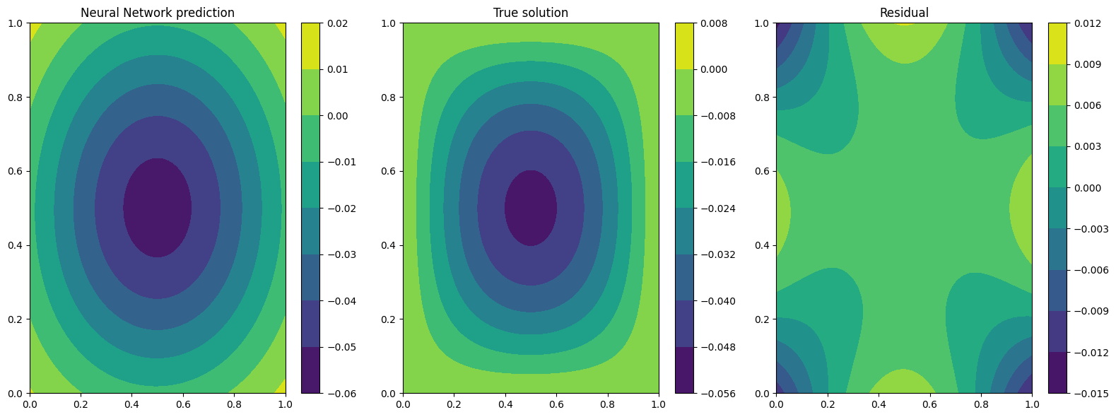
Now the Plotter class is used to plot the results. The solution
predicted by the neural network is plotted on the left, the exact one is
represented at the center and on the right the error between the exact
and the predicted solutions is showed.
plotter = Plotter()
plotter.plot(solver=pinn)

Solving the problem with extra-features PINNs#
Now, the same problem is solved in a different way. A new neural network is now defined, with an additional input variable, named extra-feature, which coincides with the forcing term in the Laplace equation. The set of input variables to the neural network is:
where \(x\) and \(y\) are the spatial coordinates and \(k(x, y)\) is the added feature.
This feature is initialized in the class SinSin, which needs to be
inherited by the torch.nn.Module class and to have the forward
method. After declaring such feature, we can just incorporate in the
FeedForward class thanks to the extra_features argument. NB:
extra_features always needs a list as input, you you have one
feature just encapsulated it in a class, as in the next cell.
Finally, we perform the same training as before: the problem is
Poisson, the network is composed by the same number of neurons and
optimizer parameters are equal to previous test, the only change is the
new extra feature.
class SinSin(torch.nn.Module):
    """Feature: sin(x)*sin(y)"""
    def __init__(self):
        super().__init__()

    def forward(self, x):
        t = (torch.sin(x.extract(['x'])*torch.pi) *
             torch.sin(x.extract(['y'])*torch.pi))
        return LabelTensor(t, ['sin(x)sin(y)'])


# make model + solver + trainer
model_feat = FeedForward(
    layers=[10, 10],
    func=Softplus,
    output_dimensions=len(problem.output_variables),
    input_dimensions=len(problem.input_variables)+1
)
pinn_feat = PINN(problem, model_feat, extra_features=[SinSin()], optimizer_kwargs={'lr':0.006, 'weight_decay':1e-8})
trainer_feat = Trainer(pinn_feat, max_epochs=1000, callbacks=[MetricTracker()], accelerator='cpu', enable_model_summary=False) # we train on CPU and avoid model summary at beginning of training (optional)

# train
trainer_feat.train()
Trainer.fit stopped: max_epochs=1000 reached.
Epoch 999: : 1it [00:00, 85.62it/s, v_num=4, gamma1_loss=2.54e-7, gamma2_loss=2.17e-7, gamma3_loss=1.94e-7, gamma4_loss=2.69e-7, D_loss=9.2e-6, mean_loss=2.03e-6]
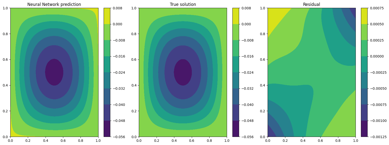
The predicted and exact solutions and the error between them are represented below. We can easily note that now our network, having almost the same condition as before, is able to reach additional order of magnitudes in accuracy.
plotter.plot(solver=pinn_feat)

Solving the problem with learnable extra-features PINNs#
We can still do better!
Another way to exploit the extra features is the addition of learnable parameter inside them. In this way, the added parameters are learned during the training phase of the neural network. In this case, we use:
where \(\alpha\) and \(\beta\) are the abovementioned
parameters. Their implementation is quite trivial: by using the class
torch.nn.Parameter we cam define all the learnable parameters we
need, and they are managed by autograd module!
class SinSinAB(torch.nn.Module):
    """ """
    def __init__(self):
        super().__init__()
        self.alpha = torch.nn.Parameter(torch.tensor([1.0]))
        self.beta = torch.nn.Parameter(torch.tensor([1.0]))


    def forward(self, x):
        t =  (
            self.beta*torch.sin(self.alpha*x.extract(['x'])*torch.pi)*
                      torch.sin(self.alpha*x.extract(['y'])*torch.pi)
        )
        return LabelTensor(t, ['b*sin(a*x)sin(a*y)'])


# make model + solver + trainer
model_lean= FeedForward(
    layers=[10, 10],
    func=Softplus,
    output_dimensions=len(problem.output_variables),
    input_dimensions=len(problem.input_variables)+1
)
pinn_lean = PINN(problem, model_lean, extra_features=[SinSinAB()], optimizer_kwargs={'lr':0.006, 'weight_decay':1e-8})
trainer_learn = Trainer(pinn_lean, max_epochs=1000, accelerator='cpu', enable_model_summary=False) # we train on CPU and avoid model summary at beginning of training (optional)

# train
trainer_learn.train()
Trainer.fit stopped: max_epochs=1000 reached.
Epoch 999: : 1it [00:00, 85.94it/s, v_num=5, gamma1_loss=3.26e-8, gamma2_loss=7.84e-8, gamma3_loss=1.13e-7, gamma4_loss=3.02e-8, D_loss=2.66e-6, mean_loss=5.82e-7]
Umh, the final loss is not appreciabily better than previous model (with
static extra features), despite the usage of learnable parameters. This
is mainly due to the over-parametrization of the network: there are many
parameter to optimize during the training, and the model in unable to
understand automatically that only the parameters of the extra feature
(and not the weights/bias of the FFN) should be tuned in order to fit
our problem. A longer training can be helpful, but in this case the
faster way to reach machine precision for solving the Poisson problem is
removing all the hidden layers in the FeedForward, keeping only the
\(\alpha\) and \(\beta\) parameters of the extra feature.
# make model + solver + trainer
model_lean= FeedForward(
    layers=[],
    func=Softplus,
    output_dimensions=len(problem.output_variables),
    input_dimensions=len(problem.input_variables)+1
)
pinn_learn = PINN(problem, model_lean, extra_features=[SinSinAB()], optimizer_kwargs={'lr':0.01, 'weight_decay':1e-8})
trainer_learn = Trainer(pinn_learn, max_epochs=1000, callbacks=[MetricTracker()], accelerator='cpu', enable_model_summary=False) # we train on CPU and avoid model summary at beginning of training (optional)

# train
trainer_learn.train()
Trainer.fit stopped: max_epochs=1000 reached.
Epoch 999: : 1it [00:00, 98.81it/s, v_num=6, gamma1_loss=2.55e-16, gamma2_loss=4.76e-17, gamma3_loss=2.55e-16, gamma4_loss=4.76e-17, D_loss=1.74e-13, mean_loss=3.5e-14]
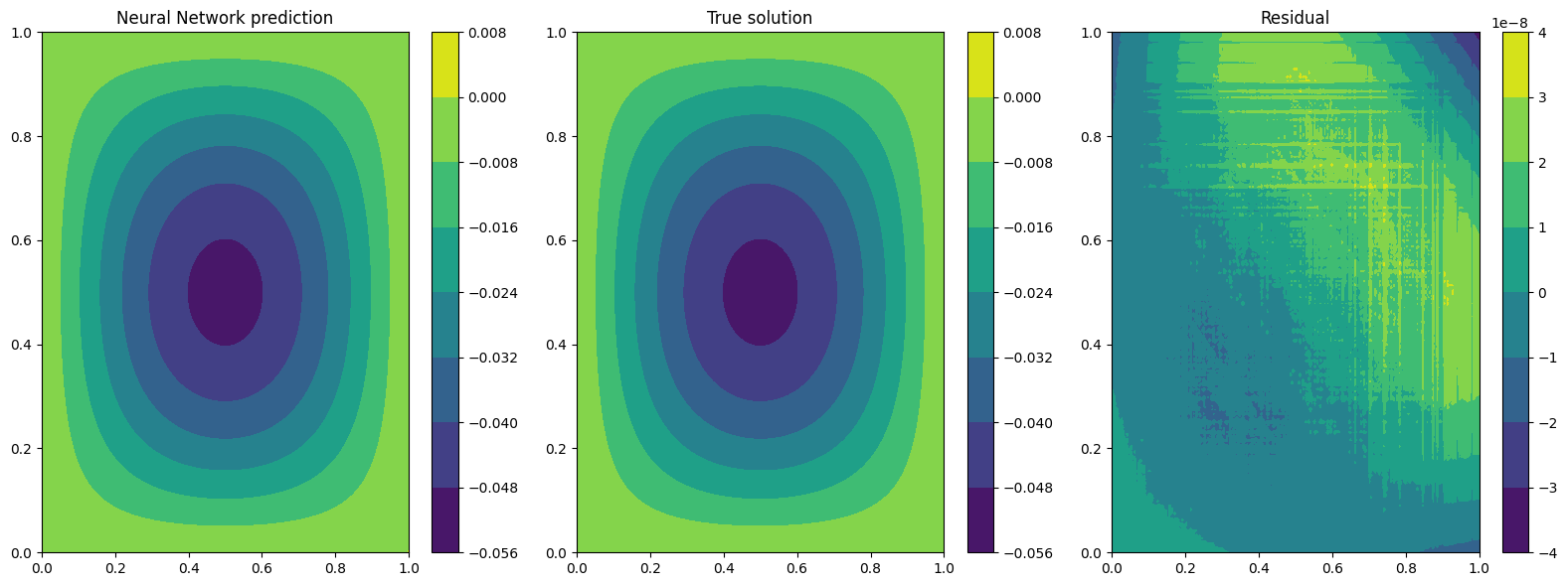
In such a way, the model is able to reach a very high accuracy! Of course, this is a toy problem for understanding the usage of extra features: similar precision could be obtained if the extra features are very similar to the true solution. The analyzed Poisson problem shows a forcing term very close to the solution, resulting in a perfect problem to address with such an approach.
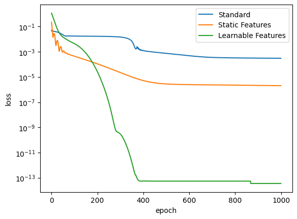
We conclude here by showing the graphical comparison of the unknown field and the loss trend for all the test cases presented here: the standard PINN, PINN with extra features, and PINN with learnable extra features.
plotter.plot(solver=pinn_learn)

Let us compare the training losses for the various types of training
plotter.plot_loss(trainer, logy=True, label='Standard')
plotter.plot_loss(trainer_feat, logy=True,label='Static Features')
plotter.plot_loss(trainer_learn, logy=True, label='Learnable Features')

What’s next?#
Nice you have completed the two dimensional Poisson tutorial of PINA! There are multiple directions you can go now:
Train the network for longer or with different layer sizes and assert the finaly accuracy
Propose new types of extrafeatures and see how they affect the learning
Exploit extrafeature training in more complex problems
Many more…
