Tutorial: Introductory Tutorial: A Beginner’s Guide to PINA

Welcome to PINA!

PINA [1] is an open-source Python library designed for Scientific Machine Learning (SciML) tasks, particularly involving:

• Physics-Informed Neural Networks (PINNs)
• Neural Operators (NOs)
• Reduced Order Models (ROMs)
• Graph Neural Networks (GNNs)
• ...

Built on PyTorch, PyTorch Lightning, and PyTorch Geometric, it provides a user-friendly, intuitive interface for formulating and solving differential problems using neural networks.

This tutorial offers a step-by-step guide to using PINA—starting from basic to advanced techniques—enabling users to tackle a broad spectrum of differential problems with minimal code.

The PINA Workflow

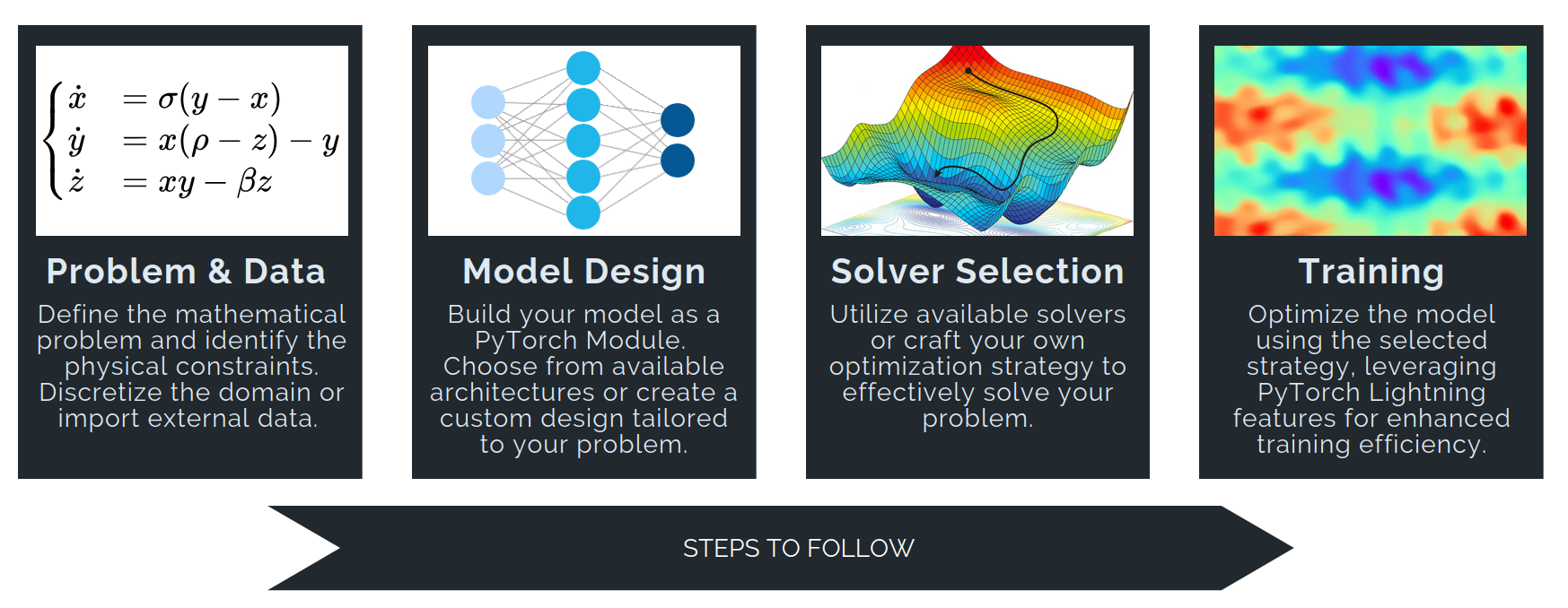
Solving a differential problem in PINA involves four main steps:

1. Problem & Data Define the mathematical problem and its physical constraints using PINA’s base classes:

   • AbstractProblem
   • SpatialProblem
   • InverseProblem
   • ...

   Then prepare inputs by discretizing the domain or importing numerical data. PINA provides essential tools like the Conditions class and the pina.domain module to facilitate domain sampling and ensure that the input data aligns with the problem's requirements.

👉 We have a dedicated tutorial to teach how to build a Problem from scratch — have a look if you're interested!

2. Model Design
   Build neural network models as PyTorch modules. For graph-structured data, use PyTorch Geometric to build Graph Neural Networks. You can also import models from pina.model module!

3. Solver Selection
   Choose and configure a solver to optimize your model. Options include:

   • Supervised solvers: SupervisedSolver, ReducedOrderModelSolver
   • Physics-informed solvers: PINN and (many) variants
   • Generative solvers: GAROM
     Solvers can be used out-of-the-box, extended, or fully customized.

4. Training
   Train your model using the Trainer class (built on PyTorch Lightning), which enables scalable and efficient training with advanced features.

By following these steps, PINA simplifies applying deep learning to scientific computing and differential problems.

A Simple Regression Problem in PINA

We'll start with a simple regression problem [2] of approximating the following function with a Neural Net model $\mathcal{M}_{\theta}$: $$y = x^3 + \epsilon, \quad \epsilon \sim \mathcal{N}(0, 9)$$
using only 20 samples:

$$x_i \sim \mathcal{U}[-3, 3], \; \forall i \in \{1, \dots, 20\}$$

Using PINA, we will:

• Generate a synthetic dataset.
• Implement a Bayesian regressor.
• Use Monte Carlo (MC) Dropout for Bayesian inference and uncertainty estimation.

This example highlights how PINA can be used for classic regression tasks with probabilistic modeling capabilities. Let's first import useful modules!

## routine needed to run the notebook on Google Colab
try:
    import google.colab

    IN_COLAB = True
except:
    IN_COLAB = False
if IN_COLAB:
    !pip install "pina-mathlab[tutorial]"

import warnings
import torch
import matplotlib.pyplot as plt

warnings.filterwarnings("ignore")

from pina import Condition, LabelTensor
from pina.problem import AbstractProblem
from pina.geometry import CartesianDomain

/opt/hostedtoolcache/Python/3.9.22/x64/lib/python3.9/site-packages/pina/geometry/__init__.py: DeprecationWarning: 'pina.geometry' is deprecated and will be removed in future versions. Please use 'pina.domain' instead. Location moved to DomainInferface object.

Problem & Data

We'll start by defining a BayesianProblem inheriting from AbstractProblem to handle input/output data. This is suitable when data is available. For other cases like PDEs without data, use:

• SpatialProblem – for spatial variables
• TimeDependentProblem – for temporal variables
• ParametricProblem – for parametric inputs
• InverseProblem – for parameter estimation from observations

but we will see this more in depth in a while!

# (a) Data generation and plot
domain = CartesianDomain({"x": [-3, 3]})
x = domain.sample(n=20, mode="random")
y = LabelTensor(x.pow(3) + 3 * torch.randn_like(x), "y")


# (b) PINA Problem formulation
class BayesianProblem(AbstractProblem):

    output_variables = ["y"]
    input_variables = ["x"]
    conditions = {"data": Condition(input_points=x, output_points=y)}


problem = BayesianProblem()

# # (b) EXTRA!
# # alternatively you can do the following which is easier
# # uncomment to try it!
# from pina.problem.zoo import SupervisedProblem
# problem = SupervisedProblem(input_=x, output_=y)

/opt/hostedtoolcache/Python/3.9.22/x64/lib/python3.9/site-packages/pina/condition/condition.py: DeprecationWarning: 'input_points' is deprecated and will be removed in future versions. Please use 'input' instead.
/opt/hostedtoolcache/Python/3.9.22/x64/lib/python3.9/site-packages/pina/condition/condition.py: DeprecationWarning: 'output_points' is deprecated and will be removed in future versions. Please use 'target' instead.

We highlight two very important features of PINA

1. LabelTensor Structure

   • Alongside the standard torch.Tensor, PINA introduces the LabelTensor structure, which allows string-based indexing.
   • Ideal for managing and stacking tensors with different labels (e.g., "x", "t", "u") for improved clarity and organization.
   • You can still use standard PyTorch tensors if needed.

2. Condition Object

   • The Condition object enforces the constraints that the model $\mathcal{M}_{\theta}$ must satisfy, such as boundary or initial conditions.
   • It ensures that the model adheres to the specific requirements of the problem, making constraint handling more intuitive and streamlined.

# EXTRA - on the use of LabelTensor

# We define a 2D tensor, and we index with ['a', 'b', 'c', 'd'] its columns
label_tensor = LabelTensor(torch.rand(3, 4), ["a", "b", "c", "d"])

print(f"The Label Tensor object, a very short introduction... \n")
print(label_tensor, "\n")
print(f"Torch methods can be used, {label_tensor.shape=}")
print(f"also {label_tensor.requires_grad=} \n")
print(f"But we have labels as well, e.g. {label_tensor.labels=}")
print(f'And we can slice with labels: \n {label_tensor["a"]=}')
print(f"Similarly to: \n {label_tensor[:, 0]=}")

The Label Tensor object, a very short introduction... 

1: {'dof': ['a', 'b', 'c', 'd'], 'name': 1}

tensor([[0.7771, 0.2222, 0.8566, 0.9572],
        [0.7311, 0.5005, 0.6676, 0.6215],
        [0.7658, 0.1562, 0.5159, 0.0455]]) 

Torch methods can be used, label_tensor.shape=torch.Size([3, 4])
also label_tensor.requires_grad=False 

But we have labels as well, e.g. label_tensor.labels=['a', 'b', 'c', 'd']
And we can slice with labels: 
 label_tensor["a"]=LabelTensor([[0.7771],
             [0.7311],
             [0.7658]])
Similarly to: 
 label_tensor[:, 0]=LabelTensor([[0.7771],
             [0.7311],
             [0.7658]])

Model Design

We will now solve the problem using a simple PyTorch Neural Network with Dropout, which we will implement from scratch following [2].
It's important to note that PINA provides a wide range of state-of-the-art (SOTA) architectures in the pina.model module, which you can explore further here.

Solver Selection

For this task, we will use a straightforward supervised learning approach by importing the SupervisedSolver from pina.solvers. The solver is responsible for defining the training strategy.

The SupervisedSolver is designed to handle typical regression tasks effectively by minimizing the following loss function: $$ \mathcal{L}_{\rm{problem}} = \frac{1}{N}\sum_{i=1}^N \mathcal{L}(y_i - \mathcal{M}_{\theta}(x_i)) $$ where $\mathcal{L}$ is the loss function, with the default being Mean Squared Error (MSE): $$ \mathcal{L}(v) = \| v \|^2_2. $$

Training

Next, we will use the Trainer class to train the model. The Trainer class, based on PyTorch Lightning, offers many features that help:

• Improve model accuracy
• Reduce training time and memory usage
• Facilitate logging and visualization

The great work done by the PyTorch Lightning team ensures a streamlined training process.

from pina.solver import SupervisedSolver
from pina.trainer import Trainer


# define problem & data (step 1)
class BayesianModel(torch.nn.Module):
    def __init__(self):
        super().__init__()
        self.layers = torch.nn.Sequential(
            torch.nn.Linear(1, 100),
            torch.nn.ReLU(),
            torch.nn.Dropout(0.5),
            torch.nn.Linear(100, 1),
        )

    def forward(self, x):
        return self.layers(x)


problem = BayesianProblem()

# model design (step 2)
model = BayesianModel()

# solver selection (step 3)
solver = SupervisedSolver(problem, model)

# training (step 4)
trainer = Trainer(solver=solver, max_epochs=2000, accelerator="cpu")
trainer.train()

You are using the plain ModelCheckpoint callback. Consider using LitModelCheckpoint which with seamless uploading to Model registry.

GPU available: False, used: False

TPU available: False, using: 0 TPU cores

HPU available: False, using: 0 HPUs

  | Name         | Type       | Params | Mode 
----------------------------------------------------
0 | _pina_models | ModuleList | 301    | train
1 | _loss_fn     | MSELoss    | 0      | train
----------------------------------------------------
301       Trainable params
0         Non-trainable params
301       Total params
0.001     Total estimated model params size (MB)
8         Modules in train mode
0         Modules in eval mode

`Trainer.fit` stopped: `max_epochs=2000` reached.

Model Training Complete! Now Visualize the Solutions

The model has been trained! Since we used Dropout during training, the model is probabilistic (Bayesian) [3]. This means that each time we evaluate the forward pass on the input points $x_i$, the results will differ due to the stochastic nature of Dropout.

To visualize the model's predictions and uncertainty, we will:

1. Evaluate the Forward Pass: Perform multiple forward passes to get different predictions for each input $x_i$.
2. Compute the Mean: Calculate the average prediction $\mu_\theta$ across all forward passes.
3. Compute the Standard Deviation: Calculate the variability of the predictions $\sigma_\theta$, which indicates the model's uncertainty.

This allows us to understand not only the predicted values but also the confidence in those predictions.

x_test = LabelTensor(torch.linspace(-4, 4, 100).reshape(-1, 1), "x")
y_test = torch.stack([solver(x_test) for _ in range(1000)], dim=0)
y_mean, y_std = y_test.mean(0).detach(), y_test.std(0).detach()
# plot
x_test = x_test.flatten()
y_mean = y_mean.flatten()
y_std = y_std.flatten()
plt.plot(x_test, y_mean, label=r"$\mu_{\theta}$")
plt.fill_between(
    x_test,
    y_mean - 3 * y_std,
    y_mean + 3 * y_std,
    alpha=0.3,
    label=r"3$\sigma_{\theta}$",
)
plt.plot(x_test, x_test.pow(3), label="true")
plt.scatter(x, y, label="train data")
plt.legend()
plt.show()

PINA for Physics-Informed Machine Learning

In the previous section, we used PINA for supervised learning. However, one of its main strengths lies in Physics-Informed Machine Learning (PIML), specifically through Physics-Informed Neural Networks (PINNs).

What Are PINNs?

PINNs are deep learning models that integrate the laws of physics directly into the training process. By incorporating differential equations and boundary conditions into the loss function, PINNs allow the modeling of complex physical systems while ensuring the predictions remain consistent with scientific laws.

Solving a 2D Poisson Problem

In this section, we will solve a 2D Poisson problem with Dirichlet boundary conditions on an hourglass-shaped domain using a simple PINN [4]. You can explore other PINN variants, e.g. [5] or [6] in PINA by visiting the PINA solvers documentation. We aim to solve the following 2D Poisson problem:

$$ \begin{cases} \Delta u(x, y) = \sin{(\pi x)} \sin{(\pi y)} & \text{in } D, \\ u(x, y) = 0 & \text{on } \partial D \end{cases} $$

where $D$ is an hourglass-shaped domain defined as the difference between a Cartesian domain and two intersecting ellipsoids, and $\partial D$ is the boundary of the domain.

Building Complex Domains

PINA allows you to build complex geometries easily. It provides many built-in domain shapes and Boolean operators for combining them. For this problem, we will define the hourglass-shaped domain using the existing CartesianDomain and EllipsoidDomain classes, with Boolean operators like Difference and Union.

👉 If you are interested in exploring the domain module in more detail, check out this tutorial.

from pina.domain import EllipsoidDomain, Difference, CartesianDomain, Union

# (a) Building the interior of the hourglass-shaped domain
cartesian = CartesianDomain({"x": [-3, 3], "y": [-3, 3]})
ellipsoid_1 = EllipsoidDomain({"x": [-5, -1], "y": [-3, 3]})
ellipsoid_2 = EllipsoidDomain({"x": [1, 5], "y": [-3, 3]})
interior = Difference([cartesian, ellipsoid_1, ellipsoid_2])

# (a) Building the boundary of the hourglass-shaped domain
border_ellipsoid_1 = EllipsoidDomain(
    {"x": [-5, -1], "y": [-3, 3]}, sample_surface=True
)
border_ellipsoid_2 = EllipsoidDomain(
    {"x": [1, 5], "y": [-3, 3]}, sample_surface=True
)
border_1 = CartesianDomain({"x": [-3, 3], "y": 3})
border_2 = CartesianDomain({"x": [-3, 3], "y": -3})
ex_1 = CartesianDomain({"x": [-5, -3], "y": [-3, 3]})
ex_2 = CartesianDomain({"x": [3, 5], "y": [-3, 3]})
border_ells = Union([border_ellipsoid_1, border_ellipsoid_2])
border = Union(
    [
        border_1,
        border_2,
        Difference(
            [Union([border_ellipsoid_1, border_ellipsoid_2]), ex_1, ex_2]
        ),
    ]
)

# (c) Sample the domains
interior_samples = interior.sample(n=1000, mode="random")
border_samples = border.sample(n=1000, mode="random")

Plotting the domain

Nice! Now that we have built the domain, let's try to plot it

plt.figure(figsize=(8, 4))
plt.subplot(1, 2, 1)
plt.scatter(
    interior_samples.extract("x"),
    interior_samples.extract("y"),
    c="blue",
    alpha=0.5,
)
plt.title("Hourglass Interior")
plt.subplot(1, 2, 2)
plt.scatter(
    border_samples.extract("x"),
    border_samples.extract("y"),
    c="blue",
    alpha=0.5,
)
plt.title("Hourglass Border")
plt.show()

Writing the Poisson Problem Class

Very good! Now we will implement the problem class for the 2D Poisson problem. Unlike the previous examples, where we inherited from AbstractProblem, for this problem, we will inherit from the SpatialProblem class.

The reason for this is that the Poisson problem involves spatial variables as input, so we use SpatialProblem to handle such cases.

This will allow us to define the problem with spatial dependencies and set up the neural network model accordingly.

from pina.problem import SpatialProblem
from pina.operator import laplacian
from pina.equation import FixedValue, Equation


def poisson_equation(input_, output_):
    force_term = torch.sin(input_.extract(["x"]) * torch.pi) * torch.sin(
        input_.extract(["y"]) * torch.pi
    )
    laplacian_u = laplacian(output_, input_, components=["u"], d=["x", "y"])
    return laplacian_u - force_term


class Poisson(SpatialProblem):
    # define output_variables and spatial_domain
    output_variables = ["u"]
    spatial_domain = Union([interior, border])
    # define the domains
    domains = {"border": border, "interior": interior}
    # define the conditions
    conditions = {
        "border": Condition(domain="border", equation=FixedValue(0.0)),
        "interior": Condition(
            domain="interior", equation=Equation(poisson_equation)
        ),
    }


poisson_problem = Poisson()

As you can see, writing the problem class for a differential equation in PINA is straightforward! The main differences are:

• We inherit from SpatialProblem instead of AbstractProblem to account for spatial variables.
• We use domain and equation inside the Condition to define the problem.

The Equation class can be very useful for creating modular problem classes. If you're interested, check out this tutorial for more details. There's also a dedicated tutorial for building custom problems!

Once the problem class is set, we need to sample the domain to obtain the data. PINA will automatically handle this, and if you forget to sample, an error will be raised before training begins 😉.

print("Points are not automatically sampled, you can see this by:")
print(f"    {poisson_problem.are_all_domains_discretised=}\n")
print("But you can easily sample by running .discretise_domain:")
poisson_problem.discretise_domain(n=1000, domains=["interior"])
poisson_problem.discretise_domain(n=100, domains=["border"])
print(f"    {poisson_problem.are_all_domains_discretised=}")

Points are not automatically sampled, you can see this by:
    poisson_problem.are_all_domains_discretised=False

But you can easily sample by running .discretise_domain:

    poisson_problem.are_all_domains_discretised=True

Building the Model

After setting the problem and sampling the domain, the next step is to build the model $\mathcal{M}_{\theta}$.

For this, we will use the custom PINA models available here. Specifically, we will use a feed-forward neural network by importing the FeedForward class.

This neural network takes the coordinates (in this case ['x', 'y']) as input and outputs the unknown field of the Poisson problem.

In this tutorial, the neural network is composed of 2 hidden layers, each with 120 neurons and tanh activation.

from pina.model import FeedForward

model = FeedForward(
    func=torch.nn.Tanh,
    layers=[120] * 2,
    output_dimensions=len(poisson_problem.output_variables),
    input_dimensions=len(poisson_problem.input_variables),
)

Solver Selection

The thir part of the PINA pipeline involves using a Solver.

In this tutorial, we will use the classical PINN solver. However, many other variants are also available and we invite to try them!

Loss Function in PINA

The loss function in the classical PINN is defined as follows:

$$\theta_{\rm{best}}=\min_{\theta}\mathcal{L}_{\rm{problem}}(\theta), \quad \mathcal{L}_{\rm{problem}}(\theta)= \frac{1}{N_{D}}\sum_{i=1}^N \mathcal{L}(\Delta\mathcal{M}_{\theta}(\mathbf{x}_i, \mathbf{y}_i) - \sin(\pi x_i)\sin(\pi y_i)) + \frac{1}{N}\sum_{i=1}^N \mathcal{L}(\mathcal{M}_{\theta}(\mathbf{x}_i, \mathbf{y}_i))$$

This loss consists of:

1. The differential equation residual: Ensures the model satisfies the Poisson equation.
2. The boundary condition: Ensures the model satisfies the Dirichlet boundary condition.

Training

For the last part of the pipeline we need a Trainer. We will train the model for 1000 epochs using the default optimizer parameters. These parameters can be adjusted as needed. For more details, check the solvers documentation here.

To track metrics during training, we use the MetricTracker class.

👉 Want to know more about Trainer and how to boost PINA performance, check out this tutorial.

from pina.solver import PINN
from pina.callback import MetricTracker

# define the solver
solver = PINN(poisson_problem, model)

# define trainer
trainer = Trainer(
    solver,
    max_epochs=1500,
    callbacks=[MetricTracker()],
    accelerator="cpu",
    enable_model_summary=False,
)

# train
trainer.train()

You are using the plain ModelCheckpoint callback. Consider using LitModelCheckpoint which with seamless uploading to Model registry.

GPU available: False, used: False

TPU available: False, using: 0 TPU cores

HPU available: False, using: 0 HPUs

`Trainer.fit` stopped: `max_epochs=1500` reached.

Done! We can plot the solution and its residual

# sample points in the domain. remember to set requires_grad!
pts = poisson_problem.spatial_domain.sample(1000).requires_grad_(True)
# compute the solution
solution = solver(pts)
# compute the residual in the interior
equation = poisson_problem.conditions["interior"].equation
residual = solver.compute_residual(pts, equation)
# simple plot
with torch.no_grad():
    plt.subplot(1, 2, 1)
    plt.scatter(
        pts.extract("x").flatten(),
        pts.extract("y").flatten(),
        c=solution.extract("u").flatten(),
    )
    plt.colorbar()
    plt.title("Solution")
    plt.subplot(1, 2, 2)
    plt.scatter(
        pts.extract("x").flatten(),
        pts.extract("y").flatten(),
        c=residual.flatten(),
    )
    plt.colorbar()
    plt.tight_layout()
    plt.title("Residual")

What's Next?

Congratulations on completing the introductory tutorial of PINA! Now that you have a solid foundation, here are a few directions you can explore:

1. Explore Advanced Solvers: Dive into more advanced solvers like SAPINN or RBAPINN and experiment with different variations of Physics-Informed Neural Networks.

2. Apply PINA to New Problems: Try solving other types of differential equations or explore inverse problems and parametric problems using the PINA framework.

3. Optimize Model Performance: Use the Trainer class to enhance model performance by exploring features like dynamic learning rates, early stopping, and model checkpoints.

4. ...and many more! — There are countless directions to further explore, from testing on different problems to refining the model architecture!

For more resources and tutorials, check out the PINA Documentation.

References

[1] Coscia, Dario, et al. "Physics-informed neural networks for advanced modeling." Journal of Open Source Software, 2023.

[2] Hernández-Lobato, José Miguel, and Ryan Adams. "Probabilistic backpropagation for scalable learning of bayesian neural networks." International conference on machine learning, 2015.

[3] Gal, Yarin, and Zoubin Ghahramani. "Dropout as a bayesian approximation: Representing model uncertainty in deep learning." International conference on machine learning, 2016.

[4] Raissi, Maziar, Paris Perdikaris, and George E. Karniadakis. "Physics-informed neural networks: A deep learning framework for solving forward and inverse problems involving nonlinear partial differential equations." Journal of Computational Physics, 2019.

[5] McClenny, Levi D., and Ulisses M. Braga-Neto. "Self-adaptive physics-informed neural networks." Journal of Computational Physics, 2023.

[6] Anagnostopoulos, Sokratis J., et al. "Residual-based attention in physics-informed neural networks." Computer Methods in Applied Mechanics and Engineering, 2024.