Tutorial: Introduction to Trainer class

In this tutorial, we will delve deeper into the functionality of the Trainer class, which serves as the cornerstone for training PINA Solvers.

The Trainer class offers a plethora of features aimed at improving model accuracy, reducing training time and memory usage, facilitating logging visualization, and more thanks to the amazing job done by the PyTorch Lightning team!

Our leading example will revolve around solving a simple regression problem where we want to approximate the following function with a Neural Net model $\mathcal{M}_{\theta}$: $$y = x^3$$ by having only a set of $20$ observations $\{x_i, y_i\}_{i=1}^{20}$, with $x_i \sim\mathcal{U}[-3, 3]\;\;\forall i\in(1,\dots,20)$.

Let's start by importing useful modules!

try:
    import google.colab

    IN_COLAB = True
except:
    IN_COLAB = False
if IN_COLAB:
    !pip install "pina-mathlab[tutorial]"

import torch
import warnings

from pina import Trainer
from pina.solver import SupervisedSolver
from pina.model import FeedForward
from pina.problem.zoo import SupervisedProblem

warnings.filterwarnings("ignore")

Define problem and solver.

# defining the problem
x_train = torch.empty((20, 1)).uniform_(-3, 3)
y_train = x_train.pow(3) + 3 * torch.randn_like(x_train)

problem = SupervisedProblem(x_train, y_train)

# build the model
model = FeedForward(
    layers=[10, 10],
    func=torch.nn.Tanh,
    output_dimensions=1,
    input_dimensions=1,
)

# create the SupervisedSolver object
solver = SupervisedSolver(problem, model, use_lt=False)

Till now we just followed the extact step of the previous tutorials. The Trainer object can be initialized by simiply passing the SupervisedSolver solver

trainer = Trainer(solver=solver)

You are using the plain ModelCheckpoint callback. Consider using LitModelCheckpoint which with seamless uploading to Model registry.

GPU available: False, used: False

TPU available: False, using: 0 TPU cores

HPU available: False, using: 0 HPUs

Trainer Accelerator

When creating the Trainer, by default the most performing accelerator for training which is available in your system will be chosen, ranked as follows:

1. TPU
2. IPU
3. HPU
4. GPU or MPS
5. CPU

For setting manually the accelerator run:

• accelerator = {'gpu', 'cpu', 'hpu', 'mps', 'cpu', 'ipu'} sets the accelerator to a specific one

trainer = Trainer(solver=solver, accelerator="cpu")

You are using the plain ModelCheckpoint callback. Consider using LitModelCheckpoint which with seamless uploading to Model registry.

GPU available: False, used: False

TPU available: False, using: 0 TPU cores

HPU available: False, using: 0 HPUs

As you can see, even if a GPU is available on the system, it is not used since we set accelerator='cpu'.

Trainer Logging

In PINA you can log metrics in different ways. The simplest approach is to use the MetricTracker class from pina.callbacks, as seen in the Introduction to Physics Informed Neural Networks training tutorial.

However, especially when we need to train multiple times to get an average of the loss across multiple runs, lightning.pytorch.loggers might be useful. Here we will use TensorBoardLogger (more on logging here), but you can choose the one you prefer (or make your own one).

We will now import TensorBoardLogger, do three runs of training, and then visualize the results. Notice we set enable_model_summary=False to avoid model summary specifications (e.g. number of parameters); set it to True if needed.

from lightning.pytorch.loggers import TensorBoardLogger

# three run of training, by default it trains for 1000 epochs, we set the max to 100
# we reinitialize the model each time otherwise the same parameters will be optimized
for _ in range(3):
    model = FeedForward(
        layers=[10, 10],
        func=torch.nn.Tanh,
        output_dimensions=1,
        input_dimensions=1,
    )
    solver = SupervisedSolver(problem, model, use_lt=False)
    trainer = Trainer(
        solver=solver,
        accelerator="cpu",
        logger=TensorBoardLogger(save_dir="training_log"),
        enable_model_summary=False,
        train_size=1.0,
        val_size=0.0,
        test_size=0.0,
        max_epochs=100,
    )
    trainer.train()

You are using the plain ModelCheckpoint callback. Consider using LitModelCheckpoint which with seamless uploading to Model registry.

GPU available: False, used: False

TPU available: False, using: 0 TPU cores

HPU available: False, using: 0 HPUs

`Trainer.fit` stopped: `max_epochs=100` reached.

You are using the plain ModelCheckpoint callback. Consider using LitModelCheckpoint which with seamless uploading to Model registry.

GPU available: False, used: False

TPU available: False, using: 0 TPU cores

HPU available: False, using: 0 HPUs

`Trainer.fit` stopped: `max_epochs=100` reached.

You are using the plain ModelCheckpoint callback. Consider using LitModelCheckpoint which with seamless uploading to Model registry.

GPU available: False, used: False

TPU available: False, using: 0 TPU cores

HPU available: False, using: 0 HPUs

`Trainer.fit` stopped: `max_epochs=100` reached.

We can now visualize the logs by simply running tensorboard --logdir=training_log/ in the terminal. You should obtain a webpage similar to the one shown below if running for 1000 epochs:

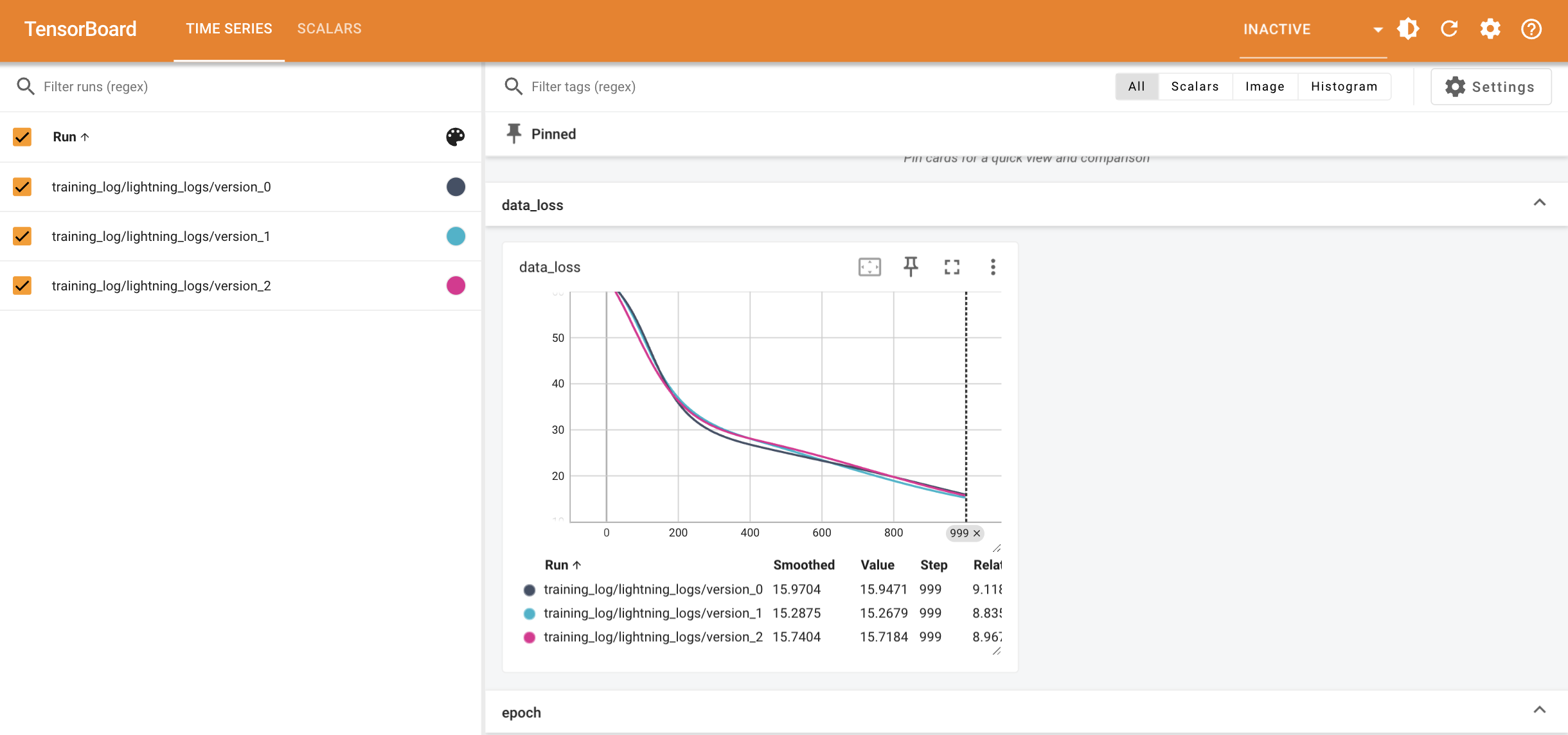
As you can see, by default, PINA logs the losses which are shown in the progress bar, as well as the number of epochs. You can always insert more loggings by either defining a callback (more on callbacks), or inheriting the solver and modifying the programs with different hooks (more on hooks).

Trainer Callbacks

Whenever we need to access certain steps of the training for logging, perform static modifications (i.e. not changing the Solver), or update Problem hyperparameters (static variables), we can use Callbacks. Notice that Callbacks allow you to add arbitrary self-contained programs to your training. At specific points during the flow of execution (hooks), the Callback interface allows you to design programs that encapsulate a full set of functionality. It de-couples functionality that does not need to be in PINA Solvers.

Lightning has a callback system to execute them when needed. Callbacks should capture NON-ESSENTIAL logic that is NOT required for your lightning module to run.

The following are best practices when using/designing callbacks:

• Callbacks should be isolated in their functionality.
• Your callback should not rely on the behavior of other callbacks in order to work properly.
• Do not manually call methods from the callback.
• Directly calling methods (e.g., on_validation_end) is strongly discouraged.
• Whenever possible, your callbacks should not depend on the order in which they are executed.

We will try now to implement a naive version of MetricTraker to show how callbacks work. Notice that this is a very easy application of callbacks, fortunately in PINA we already provide more advanced callbacks in pina.callbacks.

from lightning.pytorch.callbacks import Callback
from lightning.pytorch.callbacks import EarlyStopping
import torch


# define a simple callback
class NaiveMetricTracker(Callback):
    def __init__(self):
        self.saved_metrics = []

    def on_train_epoch_end(
        self, trainer, __
    ):  # function called at the end of each epoch
        self.saved_metrics.append(
            {key: value for key, value in trainer.logged_metrics.items()}
        )

Let's see the results when applied to the problem. You can define callbacks when initializing the Trainer by using the callbacks argument, which expects a list of callbacks.

model = FeedForward(
    layers=[10, 10],
    func=torch.nn.Tanh,
    output_dimensions=1,
    input_dimensions=1,
)
solver = SupervisedSolver(problem, model, use_lt=False)
trainer = Trainer(
    solver=solver,
    accelerator="cpu",
    logger=True,
    callbacks=[NaiveMetricTracker()],  # adding a callbacks
    enable_model_summary=False,
    train_size=1.0,
    val_size=0.0,
    test_size=0.0,
    max_epochs=10,  # training only for 10 epochs
)
trainer.train()

You are using the plain ModelCheckpoint callback. Consider using LitModelCheckpoint which with seamless uploading to Model registry.

GPU available: False, used: False

TPU available: False, using: 0 TPU cores

HPU available: False, using: 0 HPUs

`Trainer.fit` stopped: `max_epochs=10` reached.

We can easily access the data by calling trainer.callbacks[0].saved_metrics (notice the zero representing the first callback in the list given at initialization).

trainer.callbacks[0].saved_metrics[:3]  # only the first three epochs

[{'data_loss': tensor(125.5571), 'train_loss': tensor(125.5571)},
 {'data_loss': tensor(125.4812), 'train_loss': tensor(125.4812)},
 {'data_loss': tensor(125.4055), 'train_loss': tensor(125.4055)}]

PyTorch Lightning also has some built-in Callbacks which can be used in PINA, here is an extensive list.

We can, for example, try the EarlyStopping routine, which automatically stops the training when a specific metric converges (here the train_loss). In order to let the training keep going forever, set max_epochs=-1.

model = FeedForward(
    layers=[10, 10],
    func=torch.nn.Tanh,
    output_dimensions=1,
    input_dimensions=1,
)
solver = SupervisedSolver(problem, model, use_lt=False)
trainer = Trainer(
    solver=solver,
    accelerator="cpu",
    max_epochs=-1,
    enable_model_summary=False,
    enable_progress_bar=False,
    val_size=0.2,
    train_size=0.8,
    test_size=0.0,
    callbacks=[EarlyStopping("val_loss")],
)  # adding a callbacks
trainer.train()

You are using the plain ModelCheckpoint callback. Consider using LitModelCheckpoint which with seamless uploading to Model registry.

GPU available: False, used: False

TPU available: False, using: 0 TPU cores

HPU available: False, using: 0 HPUs

As we can see the model automatically stop when the logging metric stopped improving!

Trainer Tips to Boost Accuracy, Save Memory and Speed Up Training

Until now we have seen how to choose the right accelerator, how to log and visualize the results, and how to interface with the program in order to add specific parts of code at specific points via callbacks. Now, we will focus on how to boost your training by saving memory and speeding it up, while maintaining the same or even better degree of accuracy!

There are several built-in methods developed in PyTorch Lightning which can be applied straightforward in PINA. Here we report some:

• Stochastic Weight Averaging to boost accuracy
• Gradient Clipping to reduce computational time (and improve accuracy)
• Gradient Accumulation to save memory consumption
• Mixed Precision Training to save memory consumption

We will just demonstrate how to use the first two and see the results compared to standard training. We use the Timer callback from pytorch_lightning.callbacks to track the times. Let's start by training a simple model without any optimization (train for 500 epochs).

from lightning.pytorch.callbacks import Timer
from lightning.pytorch import seed_everything

# setting the seed for reproducibility
seed_everything(42, workers=True)

model = FeedForward(
    layers=[10, 10],
    func=torch.nn.Tanh,
    output_dimensions=1,
    input_dimensions=1,
)

solver = SupervisedSolver(problem, model, use_lt=False)
trainer = Trainer(
    solver=solver,
    accelerator="cpu",
    deterministic=True,  # setting deterministic=True ensure reproducibility when a seed is imposed
    max_epochs=500,
    enable_model_summary=False,
    callbacks=[Timer()],
)  # adding a callbacks
trainer.train()
print(f'Total training time {trainer.callbacks[0].time_elapsed("train"):.5f} s')

Seed set to 42

You are using the plain ModelCheckpoint callback. Consider using LitModelCheckpoint which with seamless uploading to Model registry.

GPU available: False, used: False

TPU available: False, using: 0 TPU cores

HPU available: False, using: 0 HPUs

`Trainer.fit` stopped: `max_epochs=500` reached.

Total training time 5.22811 s

Now we do the same but with StochasticWeightAveraging enabled

from lightning.pytorch.callbacks import StochasticWeightAveraging

# setting the seed for reproducibility
seed_everything(42, workers=True)

model = FeedForward(
    layers=[10, 10],
    func=torch.nn.Tanh,
    output_dimensions=1,
    input_dimensions=1,
)
solver = SupervisedSolver(problem, model, use_lt=False)
trainer = Trainer(
    solver=solver,
    accelerator="cpu",
    deterministic=True,
    max_epochs=500,
    enable_model_summary=False,
    callbacks=[Timer(), StochasticWeightAveraging(swa_lrs=0.005)],
)  # adding StochasticWeightAveraging callbacks
trainer.train()
print(f'Total training time {trainer.callbacks[0].time_elapsed("train"):.5f} s')

Seed set to 42

You are using the plain ModelCheckpoint callback. Consider using LitModelCheckpoint which with seamless uploading to Model registry.

GPU available: False, used: False

TPU available: False, using: 0 TPU cores

HPU available: False, using: 0 HPUs

Swapping scheduler `ConstantLR` for `SWALR`

`Trainer.fit` stopped: `max_epochs=500` reached.

Total training time 5.49452 s

As you can see, the training time does not change at all! Notice that around epoch 350 the scheduler is switched from the defalut one ConstantLR to the Stochastic Weight Average Learning Rate (SWALR). This is because by default StochasticWeightAveraging will be activated after int(swa_epoch_start * max_epochs) with swa_epoch_start=0.7 by default. Finally, the final train_loss is lower when StochasticWeightAveraging is used.

We will now do the same but clippling the gradient to be relatively small.

# setting the seed for reproducibility
seed_everything(42, workers=True)

model = FeedForward(
    layers=[10, 10],
    func=torch.nn.Tanh,
    output_dimensions=1,
    input_dimensions=1,
)
solver = SupervisedSolver(problem, model, use_lt=False)
trainer = Trainer(
    solver=solver,
    accelerator="cpu",
    max_epochs=500,
    enable_model_summary=False,
    gradient_clip_val=0.1,  # clipping the gradient
    callbacks=[Timer(), StochasticWeightAveraging(swa_lrs=0.005)],
)
trainer.train()
print(f'Total training time {trainer.callbacks[0].time_elapsed("train"):.5f} s')

Seed set to 42

You are using the plain ModelCheckpoint callback. Consider using LitModelCheckpoint which with seamless uploading to Model registry.

GPU available: False, used: False

TPU available: False, using: 0 TPU cores

HPU available: False, using: 0 HPUs

Swapping scheduler `ConstantLR` for `SWALR`

`Trainer.fit` stopped: `max_epochs=500` reached.

Total training time 5.60755 s

As we can see, by applying gradient clipping, we were able to achieve even lower error!

What's Next?

Now you know how to use the Trainer class efficiently in PINA! There are several directions you can explore next:

1. Explore Training on Different Devices: Test training times on various devices (e.g., TPU) to compare performance.

2. Reduce Memory Costs: Experiment with mixed precision training and gradient accumulation to optimize memory usage, especially when training Neural Operators.

3. Benchmark Trainer Speed: Benchmark the training speed of the Trainer class for different precisions to identify potential optimizations.

4. ...and many more!: Consider expanding to multi-GPU setups or other advanced configurations for large-scale training.

For more resources and tutorials, check out the PINA Documentation.