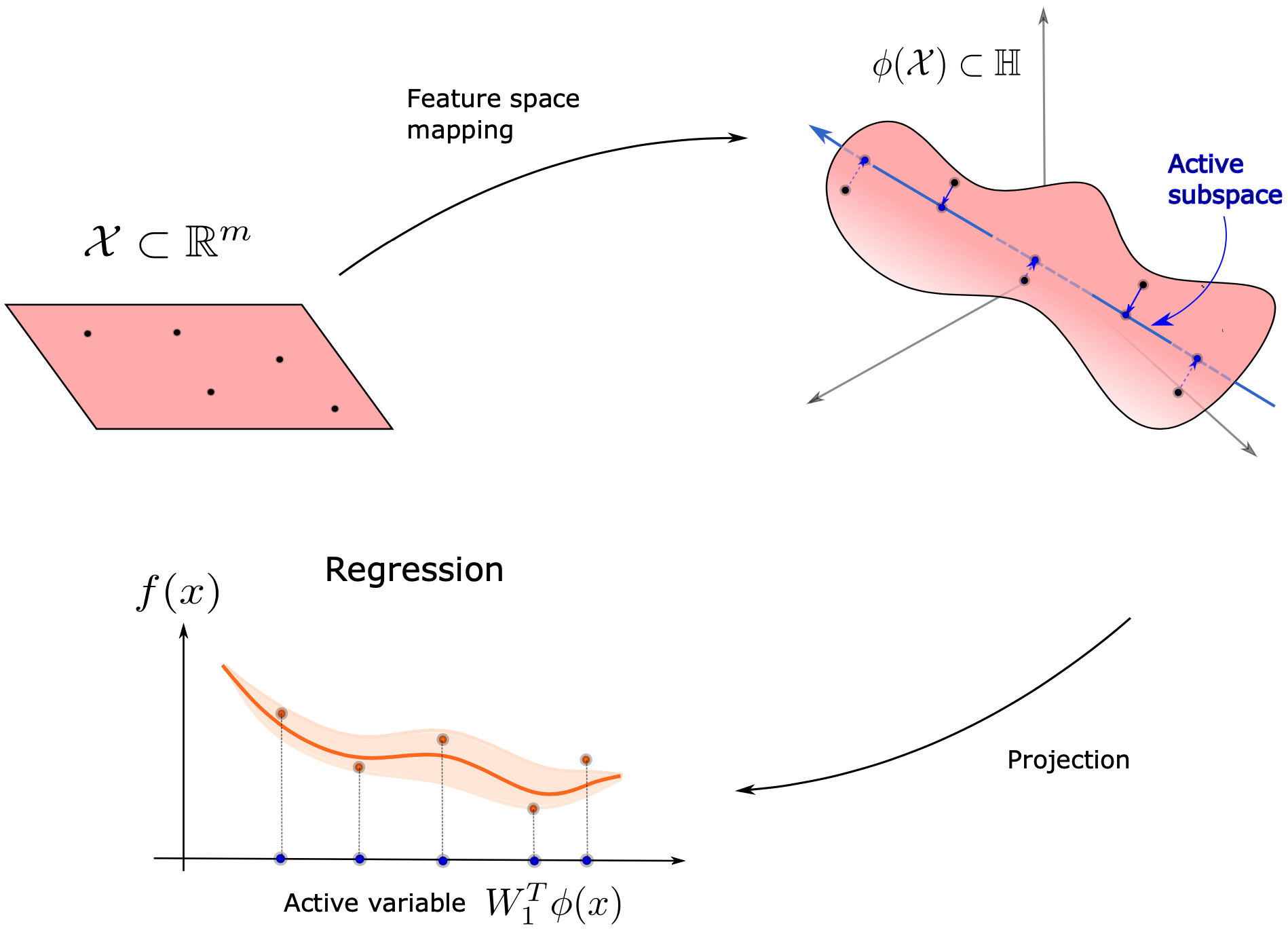
In order to extend the methodology to cases which don't have an Active Subspace, we can consider searching for a kernel-based Active Subspace.
As is common practice in Machine Learning to project the inputs from $\chi\subset\mathbb{R}^{m}$ to a Reproducing Kernel Hilbert Space (RKHS), the inputs are immersed with a feature space map $\phi$ into a supposedly infinite-dimensional Hilbert space $\phi(\chi)\subset\mathbb{H}$. Then the model function of interest factorizes over this feature map $\phi$ and a new model function $\bar{f}$ with domain the feature space
$$ f:\chi\subset\mathbb{R}^{m}\rightarrow\mathbb{R},\quad \phi:\chi\subset\mathbb{R}^{m}\rightarrow\mathbb{H}\approx\mathbb{R}^{D},\quad\bar{f}:\phi(\chi)\subset\mathbb{H}\rightarrow\mathbb{R}\\ $$$$ f = \bar{f}\circ\phi $$the RKHS $\mathbb{H}$ is approximated with a discrete feature space $\mathbb{R}^{D}$.
Searching for a kernel-based Active Subspace then reduces to finding an Active Subspace of the new model function $\bar{f}:\chi\subset\mathbb{H}\rightarrow\mathbb{R}$. In this tutorial we will consider the design of one-dimensional response functions with Gaussian process regression. A scheme of the procedure is shown below

To look more in to the details of the procedure see Kernel-based Active Subspaces with application to CFD parametric problems using Discontinuous Galerkin method. The feature map we adopt was introduced in Gaussian Process Modeling and Supervised Dimensionality Reduction Algorithms via Stiefel Manifold Learning.
import autograd.numpy as np
from autograd import elementwise_grad as egrad
import matplotlib.pyplot as plt
from functools import partial
import GPy

from athena.active import ActiveSubspaces
from athena.kas import KernelActiveSubspaces
from athena.feature_map import FeatureMap, rff_map, rff_jac
from athena.projection_factory import ProjectionFactory
from athena.utils import Normalizer, CrossValidation, average_rrmse

from numpy_functions import radial
np.random.seed(42)

# global parameters
n_samples = 800  # this is the number of data points to use for the tuning of kas
N = 500 # this is the number of test samples to use
input_dim = 2

# set the dimension of the discrete feature space (D in the introduction)
n_features = 1000
def sample_in_out(input_dim, n_samples):
    #input ranges
    lb = np.array(-3 * np.ones(input_dim))
    ub = np.array(3 * np.ones(input_dim))

    #input normalization
    XX = np.random.uniform(lb, ub, (n_samples, input_dim))

    nor = Normalizer(lb, ub)
    x = nor.fit_transform(XX)

    #output values (f) and gradients (df)
    func = partial(radial, normalizer=nor, generatrix=lambda x: np.cos(x))
    f = func(x)
    df = egrad(func)(x)
    return x, f, df
Some samples (xx, f, df) will be used for the tuning phase of the kernel-based active subspaces proceure, the remaining (y, t, dt) represents the test dataset.
xx, f, df = sample_in_out(input_dim, n_samples)
y, t, dt = sample_in_out(input_dim, N)
An active subspace is searched for, but due to the radial symmetry of the model there is no preferred direction of variation. The same result could be obtained changing the generatrix of the model. These are cases where linear active subspaces are not present and other methods should be taken in consideration.
#AS
ss = ActiveSubspaces(1)
ss.fit(gradients=dt, outputs=t, inputs=y)
ss.plot_eigenvalues(figsize=(6,4))
ss.plot_sufficient_summary(y, t, figsize=(6,4))
Define the feature map and pass it to the KernelActiveSubspaces class. The feature map is defined as
$$ \phi(\mathbf{x})=\sqrt{\frac{2}{D}}\,\sigma_f\,\cos(W\mathbf{x}+\mathbf{b}),\\ \cos(W\mathbf{x}+\mathbf{b}):=\frac{1}{\sqrt{D}}(\cos(W[1, :] \cdot \mathbf{x} +b_1),\dots, \cos(W[D, :] \cdot \mathbf{x} +b_D))^T $$where $\sigma_f$ cooresponds to the empirical variance of the model, $W\in \mathcal{M}(D\times m,\mathbb{R})$ is the projection matrix whose rows are sampled from a probability distribution on $\mathbb{R}^m$ and $\mathbf{b}\in \mathbb{R}^D$ is a bias term whose components are sampled independently and uniformly in the interval $[0, 2\pi]$.
# number of parameters of the spectral distribution associated to the feature map
# this is the number of parameters to tune after
n_params = 1

# sample the bias term
b = np.random.uniform(0, 2 * np.pi, n_features)
The list of implemented distributions to chose from is the following, the number of parameters to tune for each distribution is reported in the documentation.
ProjectionFactory.projections
['beta',
 'cauchy',
 'dirichlet',
 'laplace',
 'multivariate_normal',
 'normal',
 'uniform']
# define the feature map
fm = FeatureMap(distr='laplace',
                bias=b,
                input_dim=input_dim,
                n_features=n_features,
                params=np.zeros(n_params),
                sigma_f=f.var())

# instantiate a KernelActiveSubspaces object with associated feature map
kss = KernelActiveSubspaces(feature_map=fm, dim=1, n_features=n_features)
The feature map hyperparameters are to be tuned. Different methods are available, see the documentation. In this tutorial we will use Bayesian stochastic optimization.
# number of folds for the cross-validation algorithm
folds = 3
verbose = True
# Skip if bias and projection matrix are loaded
csv = CrossValidation(inputs=xx,
                      outputs=f.reshape(-1, 1),
                      gradients=df.reshape(n_samples, 1, input_dim),
                      folds=folds,
                      subspace=kss)
best = fm.tune_pr_matrix(func=average_rrmse,
                  bounds=[slice(-2, 0., 0.2) for i in range(n_params)],
                  fn_args={'csv':csv, 'verbose':verbose},
                  method='bso',
                  maxiter=5,
                  save_file=False)

print('The lowest rrmse is {:.3f}%'.format(best[0]*100))
################################################################################
params [0.54987828] mean 0.5806036102762929, std 0.10557747169663108
params [0.54987828] mean 0.6508088337502892, std 0.258403783743379
params [0.54987828] mean 0.5069359497235307, std 0.09170534906677469
params [0.54987828] mean 0.8635941179089066, std 0.1961446264598243
################################################################################
params [0.63303763] mean 0.7716216067211062, std 0.16253579937856896
params [0.63303763] mean 0.4363267355882392, std 0.03816486064204355
params [0.63303763] mean 0.5060488192912277, std 0.10575725753696222
params [0.63303763] mean 0.28767888162252037, std 0.04720140191709448
params [0.63303763] mean 0.5410136102749092, std 0.08078987768134094
################################################################################
params [0.04487257] mean 1.0027281038779663, std 0.0014114084641444664
################################################################################
params [0.01527761] mean 1.0006766975337171, std 0.0007903166463334343
################################################################################
params [0.02632185] mean 1.0079474661484877, std 0.0050811175188999
################################################################################
params [0.73153169] mean 1.0011729712197917, std 0.0014860539187824704
################################################################################
params [0.60876305] mean 0.9878218849767153, std 0.01783448985892262
################################################################################
params [0.63410858] mean 0.9873291014883088, std 0.022116121930394826
################################################################################
params [0.63308181] mean 1.0005712907971323, std 0.0007047386631580656
################################################################################
params [0.47263103] mean 0.9936583636821269, std 0.009511940097498308
The lowest rrmse is 28.768%
#W = np.load('opt_pr_matrix.npy')
#b = np.load('bias.npy')
#fm._pr_matrix = W
#fm.bias = b
kss.fit(gradients=dt.reshape(N, 1, input_dim),
            outputs=t,
            inputs=y)

kss.plot_eigenvalues(n_evals=5, figsize=(6,4))
kss.plot_sufficient_summary(xx, f, figsize=(6,4))
# comparison with Nonlinear Level-set Learning explained in detail in tutorial 07
from athena.nll import NonlinearLevelSet
import torch

# create NonlinearLevelSet object, eventually passing an optimizer of choice
nll = NonlinearLevelSet(n_layers=10,
                        active_dim=1,
                        lr=0.01,
                        epochs=1000,
                        dh=0.25,
                        optimizer=torch.optim.Adam)

# convert to pytorch tensors
x_torch = torch.as_tensor(xx, dtype=torch.double)
df_torch = torch.as_tensor(df, dtype=torch.double)

# train RevNet
nll.train(inputs=x_torch,
          gradients=df_torch,
          interactive=False)
epoch = 0, loss = 7.532548972955653
epoch = 10, loss = 7.221680266861894
epoch = 20, loss = 6.643592148573998
epoch = 30, loss = 6.24253642188315
epoch = 40, loss = 6.075985928347147
epoch = 50, loss = 5.9537479695453985
epoch = 60, loss = 5.8628279384482385
epoch = 70, loss = 5.845114644336895
epoch = 80, loss = 5.835431386654003
epoch = 90, loss = 5.830508028305733
epoch = 100, loss = 5.827308701073581
epoch = 110, loss = 5.824416541472429
epoch = 120, loss = 5.821889732655846
epoch = 130, loss = 5.819171229026848
epoch = 140, loss = 5.816033053439709
epoch = 150, loss = 5.811848882827806
epoch = 160, loss = 5.805241360822049
epoch = 170, loss = 5.7923747549712346
epoch = 180, loss = 5.762065173938508
epoch = 190, loss = 5.688055808002115
epoch = 200, loss = 5.571285061230882
epoch = 210, loss = 5.563880224857506
epoch = 220, loss = 5.543796546106483
epoch = 230, loss = 5.538031414804469
epoch = 240, loss = 5.535185033113964
epoch = 250, loss = 5.533332289181305
epoch = 260, loss = 5.532587489204041
epoch = 270, loss = 5.532057783857496
epoch = 280, loss = 5.531638363376278
epoch = 290, loss = 5.531268982856506
epoch = 300, loss = 5.530915371046731
epoch = 310, loss = 5.530580639574407
epoch = 320, loss = 5.530262078113562
epoch = 330, loss = 5.5299576649163455
epoch = 340, loss = 5.529666320852156
epoch = 350, loss = 5.529386745345333
epoch = 360, loss = 5.529117858349119
epoch = 370, loss = 5.528858709559586
epoch = 380, loss = 5.528608349135078
epoch = 390, loss = 5.528365802869438
epoch = 400, loss = 5.528130070891185
epoch = 410, loss = 5.527900122898406
epoch = 420, loss = 5.527674901251468
epoch = 430, loss = 5.527453322478689
epoch = 440, loss = 5.527234279955423
epoch = 450, loss = 5.527016648946539
epoch = 460, loss = 5.526799291686672
epoch = 470, loss = 5.526581062586568
epoch = 480, loss = 5.5263608124343575
epoch = 490, loss = 5.526137390939807
epoch = 500, loss = 5.525909647105348
epoch = 510, loss = 5.52567642685884
epoch = 520, loss = 5.525436567811005
epoch = 530, loss = 5.525188891587697
epoch = 540, loss = 5.524932195023223
epoch = 550, loss = 5.524665242526729
epoch = 560, loss = 5.524386762880344
epoch = 570, loss = 5.52409545428638
epoch = 580, loss = 5.523790001337072
epoch = 590, loss = 5.523469106462441
epoch = 600, loss = 5.523131536130243
epoch = 610, loss = 5.522776178648663
epoch = 620, loss = 5.522402106057409
epoch = 630, loss = 5.522008627817818
epoch = 640, loss = 5.521595319831193
epoch = 650, loss = 5.521162010335759
epoch = 660, loss = 5.520708706671569
epoch = 670, loss = 5.520235455698472
epoch = 680, loss = 5.519742145538583
epoch = 690, loss = 5.51922827233139
epoch = 700, loss = 5.518692702635283
epoch = 710, loss = 5.5181334490403104
epoch = 720, loss = 5.517547440958744
epoch = 730, loss = 5.516930227006406
epoch = 740, loss = 5.516275511212924
epoch = 750, loss = 5.515574413873817
epoch = 760, loss = 5.514814344842364
epoch = 770, loss = 5.5139773487695525
epoch = 780, loss = 5.5130376965386585
epoch = 790, loss = 5.51195833353722
epoch = 800, loss = 5.510685512902382
epoch = 810, loss = 5.509140414094771
epoch = 820, loss = 5.507205440533864
epoch = 830, loss = 5.504700394034741
epoch = 840, loss = 5.501338118018588
epoch = 850, loss = 5.496639517337872
epoch = 860, loss = 5.489799979315683
epoch = 870, loss = 5.479748125307383
epoch = 880, loss = 5.46652045173461
epoch = 890, loss = 5.453305225267302
epoch = 900, loss = 5.443000146630938
epoch = 910, loss = 5.435389483692386
epoch = 920, loss = 5.429188859742997
epoch = 930, loss = 5.423144195953234
epoch = 940, loss = 5.416715958963219
epoch = 950, loss = 5.409938251952806
epoch = 960, loss = 5.402960728929154
epoch = 970, loss = 5.39594203618684
epoch = 980, loss = 5.389094660484148
epoch = 990, loss = 5.382651715329154
epoch = 999, loss = 5.377359102673039
# loss history plot and sufficient summary plot
nll.plot_loss(figsize=(6, 4))
nll.plot_sufficient_summary(x_torch, f, figsize=(6, 4))